Debug and Optimised mode
Dear all, Is there a debug and/or optimised mode in Firedrake, to speed up the simulations? How can I access it? Thanks a lot, Floriane
On 03/03/16 10:07, Floriane Gidel [RPG] wrote:
Dear all,
Is there a debug and/or optimised mode in Firedrake, to speed up the simulations? How can I access it?
By default, you're running in, I guess "optimised" mode. However, this is a very general question and hence difficult to answer without more information. To begin with, can you send us the output of running your script passing the command-line argument "-log_summary" Thanks, Lawrence
Dear Lawrence, Thank you for your reply. The output of the command -log_summary is attached. I can also send you my code if that helps. I use a large domain with resolution of about 0.15, which might be the reason why the simulations are slow. I also need to run them for a longer time (T=80s-100s instead of T=1s in the test). Best wishes, Floriane ________________________________________ De : firedrake-bounces@imperial.ac.uk <firedrake-bounces@imperial.ac.uk> de la part de Lawrence Mitchell <lawrence.mitchell@imperial.ac.uk> Envoyé : jeudi 3 mars 2016 10:24 À : firedrake@imperial.ac.uk Objet : Re: [firedrake] Debug and Optimised mode On 03/03/16 10:07, Floriane Gidel [RPG] wrote:
Dear all,
Is there a debug and/or optimised mode in Firedrake, to speed up the simulations? How can I access it?
By default, you're running in, I guess "optimised" mode. However, this is a very general question and hence difficult to answer without more information. To begin with, can you send us the output of running your script passing the command-line argument "-log_summary" Thanks, Lawrence
On 14/03/16 11:53, Floriane Gidel [RPG] wrote:
Dear Lawrence,
Thank you for your reply. The output of the command -log_summary is attached. I can also send you my code if that helps. I use a large domain with resolution of about 0.15, which might be the reason why the simulations are slow. I also need to run them for a longer time (T=80s-100s instead of T=1s in the test).
OK, all the time is spent inside evaluating Jacobians (assembling matrices) and evaluating residuals (assembling functions). Along with quite a bit inside the solve calls. I notice that you do exactly the same number of linear solves (KSPSolve) as nonlinear solves (SNESSolve), so I suspect that your problem is linear (or at least, you have linearised "by hand" somehow). Do the operators change at every timestep? If not, you may be able to factor the solver setup (and hence save a lot of the cost) out of the timeloop. For an example of this, you can look at either the Benney-Luke demo (which does this for linear solves) http://firedrakeproject.org/demos/benney_luke.py.html. Or the Camassa-Holm demo (which uses nonlinear solves), http://firedrakeproject.org/demos/camassaholm.py.html. You say you have "high" resolution. We can try and characterise what performance you might expect to get. How many degrees of freedom are you solving for? And what kind of computer are you doing this on? You ought to be able to get some speed up just running in parallel with MPI, assuming that your computer is beefy enough. Cheers, Lawrence
Dear Lawrence, I actually solve the Benney-Luke equations so my code is very similar to the Benney-Luke demo. I define the same functions, weak formulations, problems and variational solvers. They are defined out of my time loop. Only the domain, mesh and initial conditions are different from the demo. In the time loop, I only call the solvers (e.g. eta.solve() ) and save the data. I solve it on my laptop which is a MacBook Pro with OSX version 10.9.5, and processor 2.5 GHz Intel Core i5. Best wishes, Floriane ________________________________________ De : firedrake-bounces@imperial.ac.uk <firedrake-bounces@imperial.ac.uk> de la part de Lawrence Mitchell <lawrence.mitchell@imperial.ac.uk> Envoyé : lundi 14 mars 2016 12:08 À : firedrake@imperial.ac.uk Objet : Re: [firedrake] Debug and Optimised mode On 14/03/16 11:53, Floriane Gidel [RPG] wrote:
Dear Lawrence,
Thank you for your reply. The output of the command -log_summary is attached. I can also send you my code if that helps. I use a large domain with resolution of about 0.15, which might be the reason why the simulations are slow. I also need to run them for a longer time (T=80s-100s instead of T=1s in the test).
OK, all the time is spent inside evaluating Jacobians (assembling matrices) and evaluating residuals (assembling functions). Along with quite a bit inside the solve calls. I notice that you do exactly the same number of linear solves (KSPSolve) as nonlinear solves (SNESSolve), so I suspect that your problem is linear (or at least, you have linearised "by hand" somehow). Do the operators change at every timestep? If not, you may be able to factor the solver setup (and hence save a lot of the cost) out of the timeloop. For an example of this, you can look at either the Benney-Luke demo (which does this for linear solves) http://firedrakeproject.org/demos/benney_luke.py.html. Or the Camassa-Holm demo (which uses nonlinear solves), http://firedrakeproject.org/demos/camassaholm.py.html. You say you have "high" resolution. We can try and characterise what performance you might expect to get. How many degrees of freedom are you solving for? And what kind of computer are you doing this on? You ought to be able to get some speed up just running in parallel with MPI, assuming that your computer is beefy enough. Cheers, Lawrence
On 14/03/16 12:30, Floriane Gidel [RPG] wrote:
Dear Lawrence,
I actually solve the Benney-Luke equations so my code is very similar to the Benney-Luke demo. I define the same functions, weak formulations, problems and variational solvers. They are defined out of my time loop. Only the domain, mesh and initial conditions are different from the demo. In the time loop, I only call the solvers (e.g. eta.solve() ) and save the data. I solve it on my laptop which is a MacBook Pro with OSX version 10.9.5, and processor 2.5 GHz Intel Core i5.
OK. So one thing that may well speed things up (assuming you are not already doing so) is not to output the data at every time step. I also note that the benney-luke demo uses nonlinear solvers to compute the updates: \phi^{n+1/2}, \eta^{n+1} and then \phi^{n+1}. However, the implicit equations defining these problems look to be linear in the respective implicit variables. So I think you should be able to get away with using linear solvers instead. This will mean you won't need to assemble the Jacobians all the time, but just once, which should signficantly reduce the run time. Notice that given the residual form, you can compute the appropriate Jacobian simply: Fphi_h = ... Jphi_h = derivative(Fphi_h, phi_h) If you can reformulate using linear solvers the jacobian evaluation time should drop significantly (run with -log_summary to confirm). If this turns out to be correct, we'd love a patch to the existing benney-luke demo updating it! Finally, how large is the domain? It's possible that if you want this to go much faster, once we've addressed the issues above, you'll need to run on a slightly beefier machine. Cheers, Lawrence
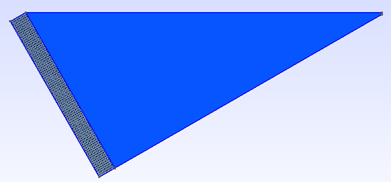
Thanks a lot Lawrence! I'll try to reformulate using linear solvers and I'll let you know how it goes. My domain has the shape of the domain attached, where the horizontal side has to be 100-300m (while the wave length is of order 1m which requires a mesh refinement of order 0.1 max). I tried to run the simulations on a faster machine but it did not improve much. But it might indeed after I linearise the solvers. I'll come back to you when it's done. Thanks a lot, Floriane ________________________________________ De : firedrake-bounces@imperial.ac.uk <firedrake-bounces@imperial.ac.uk> de la part de Lawrence Mitchell <lawrence.mitchell@imperial.ac.uk> Envoyé : lundi 14 mars 2016 13:20 À : firedrake@imperial.ac.uk Objet : Re: [firedrake] Debug and Optimised mode On 14/03/16 12:30, Floriane Gidel [RPG] wrote:
Dear Lawrence,
I actually solve the Benney-Luke equations so my code is very similar to the Benney-Luke demo. I define the same functions, weak formulations, problems and variational solvers. They are defined out of my time loop. Only the domain, mesh and initial conditions are different from the demo. In the time loop, I only call the solvers (e.g. eta.solve() ) and save the data. I solve it on my laptop which is a MacBook Pro with OSX version 10.9.5, and processor 2.5 GHz Intel Core i5.
OK. So one thing that may well speed things up (assuming you are not already doing so) is not to output the data at every time step. I also note that the benney-luke demo uses nonlinear solvers to compute the updates: \phi^{n+1/2}, \eta^{n+1} and then \phi^{n+1}. However, the implicit equations defining these problems look to be linear in the respective implicit variables. So I think you should be able to get away with using linear solvers instead. This will mean you won't need to assemble the Jacobians all the time, but just once, which should signficantly reduce the run time. Notice that given the residual form, you can compute the appropriate Jacobian simply: Fphi_h = ... Jphi_h = derivative(Fphi_h, phi_h) If you can reformulate using linear solvers the jacobian evaluation time should drop significantly (run with -log_summary to confirm). If this turns out to be correct, we'd love a patch to the existing benney-luke demo updating it! Finally, how large is the domain? It's possible that if you want this to go much faster, once we've addressed the issues above, you'll need to run on a slightly beefier machine. Cheers, Lawrence
On 14/03/16 14:22, Floriane Gidel [RPG] wrote:
Thanks a lot Lawrence! I'll try to reformulate using linear solvers and I'll let you know how it goes. My domain has the shape of the domain attached, where the horizontal side has to be 100-300m (while the wave length is of order 1m which requires a mesh refinement of order 0.1 max). I tried to run the simulations on a faster machine but it did not improve much. But it might indeed after I linearise the solvers. I'll come back to you when it's done.
Please note, looking again I see that at least the equation to compute phi^{n+1/2} *is* nonlinear, so please check my working! Lawrence
Indeed, I have used Linear Variational Solver only for eta^{n+1} and phi^{n+1} (and q^{n+1/2} ). Phi^{n+1/2} is still obtained from the NL variational solver. The new log summary is attached. Thanks, Floriane ________________________________________ De : firedrake-bounces@imperial.ac.uk <firedrake-bounces@imperial.ac.uk> de la part de Lawrence Mitchell <lawrence.mitchell@imperial.ac.uk> Envoyé : lundi 14 mars 2016 16:12 À : firedrake@imperial.ac.uk Objet : Re: [firedrake] Debug and Optimised mode On 14/03/16 14:22, Floriane Gidel [RPG] wrote:
Thanks a lot Lawrence! I'll try to reformulate using linear solvers and I'll let you know how it goes. My domain has the shape of the domain attached, where the horizontal side has to be 100-300m (while the wave length is of order 1m which requires a mesh refinement of order 0.1 max). I tried to run the simulations on a faster machine but it did not improve much. But it might indeed after I linearise the solvers. I'll come back to you when it's done.
Please note, looking again I see that at least the equation to compute phi^{n+1/2} *is* nonlinear, so please check my working! Lawrence
On 14/03/16 17:52, Floriane Gidel [RPG] wrote:
Indeed, I have used Linear Variational Solver only for eta^{n+1} and phi^{n+1} (and q^{n+1/2} ). Phi^{n+1/2} is still obtained from the NL variational solver. The new log summary is attached.
OK, this is better, we've saved about 400 seconds (out of 1200) in building jacobians. I think there is probably still some room for improvement. The computation occurs, I think, in a piecewise quadratic space (FunctionSpace(mesh, "CG", 2)). However, for output purposes, we L2-project to piecewise linears (inside file output). This can slow things down, because we repeatedly build the same projection matrix. This can especially hurt if you're outputting data at every timestep. There are two options you can use to help this, both involve writing a little more code. You need to define the piecewise linear output space yourself: V_out = FunctionSpace(mesh, "CG", 1) And the output functions, I'll only do one here: phi0_out = Function(V_out) Now, whenever you want to produce output for phi0, instead of outputting it directly, you need to first either interpolate or project it into phi0_out. With an up to date firedrake you can use either of the following (depending on whether you want interpolation or projection). For interpolation: phi0_out.interpolate(phi0) phi_out << phi0_out For projection: Outside the time loop: phi_proj = Projector(phi0, phi0_out) inside the time loop: phi_proj.project() phi_out << phi0_out If you only output very infrequently, then this is less likely to be a problem, so this may not help a huge amount. However, if the output is frequent, you might find this makes a difference. Once we've got this right, we can think about looking at the performance of the solvers. And also how much performance you might expect to be getting. Thanks, Lawrence
Dear Floriane, For the beach coupling problem in Firedrake the same remark applies when using symplectic Euler for both shallow water or Benney-Luke, and symplectic Euler for FV shallow water with flooding, in fully coupled mode: - starting with solving the continuity equation as coupled FEM and FV, this equation is linear in eta or h (note that eta can be expressed in terms of the full h too). That means that the entire coupled system is a linear system in h^n+1. The next step is nonlinear but explicit. This should simplify solving matters and thus enhance stability. Best wishes, Onno ________________________________________ From: firedrake-bounces@imperial.ac.uk <firedrake-bounces@imperial.ac.uk> on behalf of Floriane Gidel [RPG] <mmfg@leeds.ac.uk> Sent: Monday, March 14, 2016 2:22 PM To: firedrake@imperial.ac.uk Subject: Re: [firedrake] Debug and Optimised mode Thanks a lot Lawrence! I'll try to reformulate using linear solvers and I'll let you know how it goes. My domain has the shape of the domain attached, where the horizontal side has to be 100-300m (while the wave length is of order 1m which requires a mesh refinement of order 0.1 max). I tried to run the simulations on a faster machine but it did not improve much. But it might indeed after I linearise the solvers. I'll come back to you when it's done. Thanks a lot, Floriane ________________________________________ De : firedrake-bounces@imperial.ac.uk <firedrake-bounces@imperial.ac.uk> de la part de Lawrence Mitchell <lawrence.mitchell@imperial.ac.uk> Envoyé : lundi 14 mars 2016 13:20 À : firedrake@imperial.ac.uk Objet : Re: [firedrake] Debug and Optimised mode On 14/03/16 12:30, Floriane Gidel [RPG] wrote:
Dear Lawrence,
I actually solve the Benney-Luke equations so my code is very similar to the Benney-Luke demo. I define the same functions, weak formulations, problems and variational solvers. They are defined out of my time loop. Only the domain, mesh and initial conditions are different from the demo. In the time loop, I only call the solvers (e.g. eta.solve() ) and save the data. I solve it on my laptop which is a MacBook Pro with OSX version 10.9.5, and processor 2.5 GHz Intel Core i5.
OK. So one thing that may well speed things up (assuming you are not already doing so) is not to output the data at every time step. I also note that the benney-luke demo uses nonlinear solvers to compute the updates: \phi^{n+1/2}, \eta^{n+1} and then \phi^{n+1}. However, the implicit equations defining these problems look to be linear in the respective implicit variables. So I think you should be able to get away with using linear solvers instead. This will mean you won't need to assemble the Jacobians all the time, but just once, which should signficantly reduce the run time. Notice that given the residual form, you can compute the appropriate Jacobian simply: Fphi_h = ... Jphi_h = derivative(Fphi_h, phi_h) If you can reformulate using linear solvers the jacobian evaluation time should drop significantly (run with -log_summary to confirm). If this turns out to be correct, we'd love a patch to the existing benney-luke demo updating it! Finally, how large is the domain? It's possible that if you want this to go much faster, once we've addressed the issues above, you'll need to run on a slightly beefier machine. Cheers, Lawrence
Dear Lawrence, Using linear solvers indeed improved a bit the running time. Would you like me to send you the new formulations to update the demo? Concerning the non linear solver, how can I change the tolerance so that it iterates less when possible? I have another question concerning the pvd/vtu files: when saving the data with the command "<<", what is the operation applied? Is it only a linear interpolation? Because when I observe the data on Paraview and scale the colorbar to the data range for a given snapshot, the maximum value is different from the maximum value that I get if I save max(eta.dat.data), and this difference is really high (for instance, the amplitude of my wave is 2.45 with max(eta.dat.data), and 2.7 with paraview, while for this study I look at variations of order 0.01). My mesh resolution is 0.2, which is much smaller than my wave length, so even if max(eta.dat.data) takes the maximum at the grid points, I do not expect such a difference... Do you know where this difference could come from? Best wishes, Floriane ________________________________________ From: firedrake-bounces@imperial.ac.uk <firedrake-bounces@imperial.ac.uk> on behalf of Floriane Gidel [RPG] <mmfg@leeds.ac.uk> Sent: Monday, March 14, 2016 2:22 PM To: firedrake@imperial.ac.uk Subject: Re: [firedrake] Debug and Optimised mode Thanks a lot Lawrence! I'll try to reformulate using linear solvers and I'll let you know how it goes. My domain has the shape of the domain attached, where the horizontal side has to be 100-300m (while the wave length is of order 1m which requires a mesh refinement of order 0.1 max). I tried to run the simulations on a faster machine but it did not improve much. But it might indeed after I linearise the solvers. I'll come back to you when it's done. Thanks a lot, Floriane ________________________________________ De : firedrake-bounces@imperial.ac.uk <firedrake-bounces@imperial.ac.uk> de la part de Lawrence Mitchell <lawrence.mitchell@imperial.ac.uk> Envoyé : lundi 14 mars 2016 13:20 À : firedrake@imperial.ac.uk Objet : Re: [firedrake] Debug and Optimised mode On 14/03/16 12:30, Floriane Gidel [RPG] wrote:
Dear Lawrence,
I actually solve the Benney-Luke equations so my code is very similar to the Benney-Luke demo. I define the same functions, weak formulations, problems and variational solvers. They are defined out of my time loop. Only the domain, mesh and initial conditions are different from the demo. In the time loop, I only call the solvers (e.g. eta.solve() ) and save the data. I solve it on my laptop which is a MacBook Pro with OSX version 10.9.5, and processor 2.5 GHz Intel Core i5.
OK. So one thing that may well speed things up (assuming you are not already doing so) is not to output the data at every time step. I also note that the benney-luke demo uses nonlinear solvers to compute the updates: \phi^{n+1/2}, \eta^{n+1} and then \phi^{n+1}. However, the implicit equations defining these problems look to be linear in the respective implicit variables. So I think you should be able to get away with using linear solvers instead. This will mean you won't need to assemble the Jacobians all the time, but just once, which should signficantly reduce the run time. Notice that given the residual form, you can compute the appropriate Jacobian simply: Fphi_h = ... Jphi_h = derivative(Fphi_h, phi_h) If you can reformulate using linear solvers the jacobian evaluation time should drop significantly (run with -log_summary to confirm). If this turns out to be correct, we'd love a patch to the existing benney-luke demo updating it! Finally, how large is the domain? It's possible that if you want this to go much faster, once we've addressed the issues above, you'll need to run on a slightly beefier machine. Cheers, Lawrence _______________________________________________ firedrake mailing list firedrake@imperial.ac.uk https://mailman.ic.ac.uk/mailman/listinfo/firedrake
Also record the average number, min and max number of iterations. ________________________________________ From: firedrake-bounces@imperial.ac.uk <firedrake-bounces@imperial.ac.uk> on behalf of Floriane Gidel [RPG] <mmfg@leeds.ac.uk> Sent: Thursday, March 17, 2016 10:29 AM To: firedrake@imperial.ac.uk Subject: Re: [firedrake] Debug and Optimised mode Dear Lawrence, Using linear solvers indeed improved a bit the running time. Would you like me to send you the new formulations to update the demo? Concerning the non linear solver, how can I change the tolerance so that it iterates less when possible? I have another question concerning the pvd/vtu files: when saving the data with the command "<<", what is the operation applied? Is it only a linear interpolation? Because when I observe the data on Paraview and scale the colorbar to the data range for a given snapshot, the maximum value is different from the maximum value that I get if I save max(eta.dat.data), and this difference is really high (for instance, the amplitude of my wave is 2.45 with max(eta.dat.data), and 2.7 with paraview, while for this study I look at variations of order 0.01). My mesh resolution is 0.2, which is much smaller than my wave length, so even if max(eta.dat.data) takes the maximum at the grid points, I do not expect such a difference... Do you know where this difference could come from? Best wishes, Floriane ________________________________________ From: firedrake-bounces@imperial.ac.uk <firedrake-bounces@imperial.ac.uk> on behalf of Floriane Gidel [RPG] <mmfg@leeds.ac.uk> Sent: Monday, March 14, 2016 2:22 PM To: firedrake@imperial.ac.uk Subject: Re: [firedrake] Debug and Optimised mode Thanks a lot Lawrence! I'll try to reformulate using linear solvers and I'll let you know how it goes. My domain has the shape of the domain attached, where the horizontal side has to be 100-300m (while the wave length is of order 1m which requires a mesh refinement of order 0.1 max). I tried to run the simulations on a faster machine but it did not improve much. But it might indeed after I linearise the solvers. I'll come back to you when it's done. Thanks a lot, Floriane ________________________________________ De : firedrake-bounces@imperial.ac.uk <firedrake-bounces@imperial.ac.uk> de la part de Lawrence Mitchell <lawrence.mitchell@imperial.ac.uk> Envoyé : lundi 14 mars 2016 13:20 À : firedrake@imperial.ac.uk Objet : Re: [firedrake] Debug and Optimised mode On 14/03/16 12:30, Floriane Gidel [RPG] wrote:
Dear Lawrence,
I actually solve the Benney-Luke equations so my code is very similar to the Benney-Luke demo. I define the same functions, weak formulations, problems and variational solvers. They are defined out of my time loop. Only the domain, mesh and initial conditions are different from the demo. In the time loop, I only call the solvers (e.g. eta.solve() ) and save the data. I solve it on my laptop which is a MacBook Pro with OSX version 10.9.5, and processor 2.5 GHz Intel Core i5.
OK. So one thing that may well speed things up (assuming you are not already doing so) is not to output the data at every time step. I also note that the benney-luke demo uses nonlinear solvers to compute the updates: \phi^{n+1/2}, \eta^{n+1} and then \phi^{n+1}. However, the implicit equations defining these problems look to be linear in the respective implicit variables. So I think you should be able to get away with using linear solvers instead. This will mean you won't need to assemble the Jacobians all the time, but just once, which should signficantly reduce the run time. Notice that given the residual form, you can compute the appropriate Jacobian simply: Fphi_h = ... Jphi_h = derivative(Fphi_h, phi_h) If you can reformulate using linear solvers the jacobian evaluation time should drop significantly (run with -log_summary to confirm). If this turns out to be correct, we'd love a patch to the existing benney-luke demo updating it! Finally, how large is the domain? It's possible that if you want this to go much faster, once we've addressed the issues above, you'll need to run on a slightly beefier machine. Cheers, Lawrence _______________________________________________ firedrake mailing list firedrake@imperial.ac.uk https://mailman.ic.ac.uk/mailman/listinfo/firedrake _______________________________________________ firedrake mailing list firedrake@imperial.ac.uk https://mailman.ic.ac.uk/mailman/listinfo/firedrake
On 17/03/16 10:29, Floriane Gidel [RPG] wrote:
Dear Lawrence,
Using linear solvers indeed improved a bit the running time. Would you like me to send you the new formulations to update the demo?
Yes please, please create a pull request on github for your changes to the demo.
Concerning the non linear solver, how can I change the tolerance so that it iterates less when possible?
There are two types of tolerance you can control. How tightly you solve the nonlinear system, and how tightly you solve the linearisation at each nonlinear step. These can be controlled by passing solver parameters. See http://firedrakeproject.org/solving-interface.html#setting-solver-tolerances (and the matching section on nonlinear solvers on that page). Note as well that you can use Eisenstat-Walker to adaptively control the tolerance of the linear solve inside the nonlinear solver. This can be accessed using 'snes_ksp_ew': True. See https://www.mcs.anl.gov/petsc/petsc-current/docs/manualpages/SNES/SNESKSPSet... for more information.
I have another question concerning the pvd/vtu files: when saving the data with the command "<<", what is the operation applied? Is it only a linear interpolation?
No, currently it is an L_2 projection into a space of piecewise linears. We intend to switch to interpolation but have not done so yet. You can do so "by hand", I think I explained how in one of my previous emails.
Because when I observe the data on Paraview and scale the colorbar to the data range for a given snapshot, the maximum value is different from the maximum value that I get if I save max(eta.dat.data), and this difference is really high (for instance, the amplitude of my wave is 2.45 with max(eta.dat.data), and 2.7 with paraview, while for this study I look at variations of order 0.01). My mesh resolution is 0.2, which is much smaller than my wave length, so even if max(eta.dat.data) takes the maximum at the grid points, I do not expect such a difference... Do you know where this difference could come from?
It probably comes from the L_2 projection. Thanks, Lawrence
participants (3)
-
Floriane Gidel [RPG]
-
Lawrence Mitchell
-
Onno Bokhove