Nonphysical terminated simulation - CompressibleFlowSolver
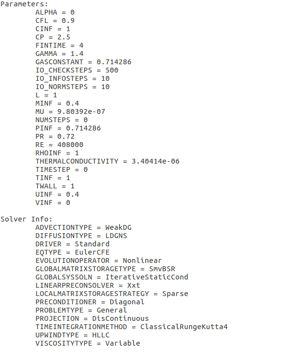
Dear users, I hope you can help one more time. I got nonphysical oscillations during my airfoil-simulation. At that time my simulations terminate with the message: "NaN found during time integration". For more information of the error and parameters see pictures below. I tried to solve this by a higher polynomial degree up to p=7 (this generates 1.5 Mio grid-points here for a 2D simulation), but the simulation terminates still. The time step itself is computed by a fixed CFL=0.9 condition. Maybe this is the wrong way, because this condition is not sufficient? So please can somebody give me a hint about that? Do I have to use another kind of grid, because the resolution of the boundary at the peak of the airfoil is not high enough or the grid lines have no be orthogonal to the surface? I am already using the spherigons-tool and tried to get a smooth boundary of my airfoil. I am using the CompressibleFlowSolver on a parallel run up to 96 CPUs by solving the Euler-Equations (EulerCFE) and the Navier-Stokes-Equations (NavierStokesCFE). The simulation terminates for both. By the way what is the difference between EulerCFE and EulerADCFE (there are no information about it anywhere)? I tried to run the example NACA0012 of the paper "Nektar++: An open-source spectral/hp element framework". The conditions use the EulerADCFE, but by running this example the simulation does not terminate, but also does not change (values of every variable in the whole domain are constant over the time - no changes?). Thanks for any help! Best regards Fabian Visualization of the grid at a polynomial degree of p=2 just before terminating: [cid:71608e01-1455-4c20-abbb-9508cb48f805] With auto-scale: [cid:bba140ce-246a-4689-a539-79ff287727b0] Same solution with scaling by user: [cid:a6bda960-d10e-4f91-a833-2e5537f8758c] Please take into account the scaling above. Error and conditions for example p=2: [cid:0ebd995c-1bae-4c43-9d08-91fe685022bf] [cid:300abb94-0f24-4dde-8cda-f67f326ea4f8] [cid:a43f5fef-3537-4385-a2d9-2f49afbcf006] Visualization of the grid at a polynomial degree of p=7 just before terminating: [cid:4d0f11c2-718a-4f85-860f-e5c90684699e] (a few time steps after that the simulation terminates and the values go against inf...)
Sorry, I forgot to note that the oscillations always take place next to the boundary of my parallelized fields (see picture below)! Maybe its an issue due to the parallelization process? There are to many possibilities about the reason of termination, so I hope somebody can give me an advice. Thanks! Best regards Fabian [cid:44c10113-782b-4fb7-a626-997b5dd94cac] (Picture shows the boundary between two parallelized fields and oscillations next to this boundary and the airfoil-surface) ________________________________ Von: nektar-users-bounces@imperial.ac.uk [nektar-users-bounces@imperial.ac.uk]" im Auftrag von "Selbach, Fabian [fabian.selbach@student.uni-siegen.de] Gesendet: Mittwoch, 30. November 2016 14:21 An: nektar-users@imperial.ac.uk Betreff: [Nektar-users] Nonphysical terminated simulation - CompressibleFlowSolver Dear users, I hope you can help one more time. I got nonphysical oscillations during my airfoil-simulation. At that time my simulations terminate with the message: "NaN found during time integration". For more information of the error and parameters see pictures below. I tried to solve this by a higher polynomial degree up to p=7 (this generates 1.5 Mio grid-points here for a 2D simulation), but the simulation terminates still. The time step itself is computed by a fixed CFL=0.9 condition. Maybe this is the wrong way, because this condition is not sufficient? So please can somebody give me a hint about that? Do I have to use another kind of grid, because the resolution of the boundary at the peak of the airfoil is not high enough or the grid lines have no be orthogonal to the surface? I am already using the spherigons-tool and tried to get a smooth boundary of my airfoil. I am using the CompressibleFlowSolver on a parallel run up to 96 CPUs by solving the Euler-Equations (EulerCFE) and the Navier-Stokes-Equations (NavierStokesCFE). The simulation terminates for both. By the way what is the difference between EulerCFE and EulerADCFE (there are no information about it anywhere)? I tried to run the example NACA0012 of the paper "Nektar++: An open-source spectral/hp element framework". The conditions use the EulerADCFE, but by running this example the simulation does not terminate, but also does not change (values of every variable in the whole domain are constant over the time - no changes?). Thanks for any help! Best regards Fabian Visualization of the grid at a polynomial degree of p=2 just before terminating: [cid:71608e01-1455-4c20-abbb-9508cb48f805] With auto-scale: [cid:bba140ce-246a-4689-a539-79ff287727b0] Same solution with scaling by user: [cid:a6bda960-d10e-4f91-a833-2e5537f8758c] Please take into account the scaling above. Error and conditions for example p=2: [cid:0ebd995c-1bae-4c43-9d08-91fe685022bf] [cid:300abb94-0f24-4dde-8cda-f67f326ea4f8] [cid:a43f5fef-3537-4385-a2d9-2f49afbcf006] Visualization of the grid at a polynomial degree of p=7 just before terminating: [cid:4d0f11c2-718a-4f85-860f-e5c90684699e] (a few time steps after that the simulation terminates and the values go against inf...)
Hi Fabian, I don't know what is causing these oscillations (maybe you need a lower CFL), but regarding your other question: EulerADCFE allows using artificial diffusion for shock capture, while EulerCFE is just the standard Euler solver. For EulerADCFE you need to set the "ShockCaptureType" property (possible values are "Smooth" and "NonSmooth") and the parameters described in section 9.4.1 of the user guide. In the most recent version of the master branch (this was changed just a few days ago), it is also possible to use shock capture directly with EulerCFE. In this newer version, EulerCFE and EulerADCFE are the same thing, with the second name kept for backwards compatibility. Cheers, Douglas ________________________________ From: nektar-users-bounces@imperial.ac.uk <nektar-users-bounces@imperial.ac.uk> on behalf of Selbach, Fabian <fabian.selbach@student.uni-siegen.de> Sent: 30 November 2016 13:21:42 To: nektar-users Subject: [Nektar-users] Nonphysical terminated simulation - CompressibleFlowSolver Dear users, I hope you can help one more time. I got nonphysical oscillations during my airfoil-simulation. At that time my simulations terminate with the message: "NaN found during time integration". For more information of the error and parameters see pictures below. I tried to solve this by a higher polynomial degree up to p=7 (this generates 1.5 Mio grid-points here for a 2D simulation), but the simulation terminates still. The time step itself is computed by a fixed CFL=0.9 condition. Maybe this is the wrong way, because this condition is not sufficient? So please can somebody give me a hint about that? Do I have to use another kind of grid, because the resolution of the boundary at the peak of the airfoil is not high enough or the grid lines have no be orthogonal to the surface? I am already using the spherigons-tool and tried to get a smooth boundary of my airfoil. I am using the CompressibleFlowSolver on a parallel run up to 96 CPUs by solving the Euler-Equations (EulerCFE) and the Navier-Stokes-Equations (NavierStokesCFE). The simulation terminates for both. By the way what is the difference between EulerCFE and EulerADCFE (there are no information about it anywhere)? I tried to run the example NACA0012 of the paper "Nektar++: An open-source spectral/hp element framework". The conditions use the EulerADCFE, but by running this example the simulation does not terminate, but also does not change (values of every variable in the whole domain are constant over the time - no changes?). Thanks for any help! Best regards Fabian Visualization of the grid at a polynomial degree of p=2 just before terminating: [cid:71608e01-1455-4c20-abbb-9508cb48f805] With auto-scale: [cid:bba140ce-246a-4689-a539-79ff287727b0] Same solution with scaling by user: [cid:a6bda960-d10e-4f91-a833-2e5537f8758c] Please take into account the scaling above. Error and conditions for example p=2: [cid:0ebd995c-1bae-4c43-9d08-91fe685022bf] [cid:300abb94-0f24-4dde-8cda-f67f326ea4f8] [cid:a43f5fef-3537-4385-a2d9-2f49afbcf006] Visualization of the grid at a polynomial degree of p=7 just before terminating: [cid:4d0f11c2-718a-4f85-860f-e5c90684699e] (a few time steps after that the simulation terminates and the values go against inf...)
Hi Douglas, Dear users, thanks for your explanation of the EulerADCFE. Your hint to decrease the CFL does not help to stabilize the simulation. Also decreasing the time step on my own to a very small one (analogical CFL=0.4) and to use another time integration method makes no difference. The simulation terminates at the same time. But I observed, that using less CPUs for parallel simulation helps to remain stable for a longer time, but finally it terminates too. Could it be a problem due to parallelization? I will try to generate a new and better grid, because this is the last clue I got. Has somebody else an idea what could causes this oscillations? Thanks in advance! Best regards Fabian ________________________________ Von: Serson, Douglas [d.serson14@imperial.ac.uk] Gesendet: Mittwoch, 30. November 2016 15:17 An: Selbach, Fabian; nektar-users Betreff: Re: [Nektar-users] Nonphysical terminated simulation - CompressibleFlowSolver Hi Fabian, I don't know what is causing these oscillations (maybe you need a lower CFL), but regarding your other question: EulerADCFE allows using artificial diffusion for shock capture, while EulerCFE is just the standard Euler solver. For EulerADCFE you need to set the "ShockCaptureType" property (possible values are "Smooth" and "NonSmooth") and the parameters described in section 9.4.1 of the user guide. In the most recent version of the master branch (this was changed just a few days ago), it is also possible to use shock capture directly with EulerCFE. In this newer version, EulerCFE and EulerADCFE are the same thing, with the second name kept for backwards compatibility. Cheers, Douglas ________________________________ From: nektar-users-bounces@imperial.ac.uk <nektar-users-bounces@imperial.ac.uk> on behalf of Selbach, Fabian <fabian.selbach@student.uni-siegen.de> Sent: 30 November 2016 13:21:42 To: nektar-users Subject: [Nektar-users] Nonphysical terminated simulation - CompressibleFlowSolver Dear users, I hope you can help one more time. I got nonphysical oscillations during my airfoil-simulation. At that time my simulations terminate with the message: "NaN found during time integration". For more information of the error and parameters see pictures below. I tried to solve this by a higher polynomial degree up to p=7 (this generates 1.5 Mio grid-points here for a 2D simulation), but the simulation terminates still. The time step itself is computed by a fixed CFL=0.9 condition. Maybe this is the wrong way, because this condition is not sufficient? So please can somebody give me a hint about that? Do I have to use another kind of grid, because the resolution of the boundary at the peak of the airfoil is not high enough or the grid lines have no be orthogonal to the surface? I am already using the spherigons-tool and tried to get a smooth boundary of my airfoil. I am using the CompressibleFlowSolver on a parallel run up to 96 CPUs by solving the Euler-Equations (EulerCFE) and the Navier-Stokes-Equations (NavierStokesCFE). The simulation terminates for both. By the way what is the difference between EulerCFE and EulerADCFE (there are no information about it anywhere)? I tried to run the example NACA0012 of the paper "Nektar++: An open-source spectral/hp element framework". The conditions use the EulerADCFE, but by running this example the simulation does not terminate, but also does not change (values of every variable in the whole domain are constant over the time - no changes?). Thanks for any help! Best regards Fabian Visualization of the grid at a polynomial degree of p=2 just before terminating: [cid:71608e01-1455-4c20-abbb-9508cb48f805] With auto-scale: [cid:bba140ce-246a-4689-a539-79ff287727b0] Same solution with scaling by user: [cid:a6bda960-d10e-4f91-a833-2e5537f8758c] Please take into account the scaling above. Error and conditions for example p=2: [cid:0ebd995c-1bae-4c43-9d08-91fe685022bf] [cid:300abb94-0f24-4dde-8cda-f67f326ea4f8] [cid:a43f5fef-3537-4385-a2d9-2f49afbcf006] Visualization of the grid at a polynomial degree of p=7 just before terminating: [cid:4d0f11c2-718a-4f85-860f-e5c90684699e] (a few time steps after that the simulation terminates and the values go against inf...)
Hi Fabian, Thanks for getting in touch and apologies for the slow response. I have a few thoughts that might help. - I would say that from your pictures, the meshes look very coarse, so you could definitely try some additional refinement. - Another source of instability can arise through the default quadrature points being used for inner products etc. You might find that using a more consistent integration could help, particularly if the grid is not well resolved. Depending on your mesh and setup, you can use an expansion tag like: <E COMPOSITE=“C[0]” BASISTYPE=“Modified_A,Modified_A" NUMMODES="3,3" POINTSTYPE="GaussLobattoLegendre,GaussLobattoLegendre" NUMPOINTS="6,6" FIELDS="rho,rhou,rhov,E" /> Note that this would use a polynomial order of 2 (nummodes = 3) whilst using double the number of grid points for integration (numpoints = 6) -- the default is one extra (numpoints = 4) which is generally sufficient but in the case of marginal resolution may lead to significant aliasing error. It'll therefore be more expensive but may be more robust. - I am not sure our CFL estimate for the compressible solver is all that great, so I would probably stick to a constant timestep, at least in the short term to investigate the reason for this instability. This is something we need to work on. - You should be aware that for these explicit schemes, larger polynomial orders will have a greater impact on the size of the maximum timestep, so perhaps best to limit to p=3-5 -- p=7 might be a bit restrictive on the timestep. It is probably better to try a grid refinement rather than increase the polynomial order. If none of this helps we can also see if Gianmarco has some input since he has run these cases extensively during his PhD and encountered may similar problems! Cheers, Dave
On 2 Dec 2016, at 09:53, Selbach, Fabian <fabian.selbach@student.uni-siegen.de> wrote:
Hi Douglas, Dear users,
thanks for your explanation of the EulerADCFE.
Your hint to decrease the CFL does not help to stabilize the simulation. Also decreasing the time step on my own to a very small one (analogical CFL=0.4) and to use another time integration method makes no difference. The simulation terminates at the same time. But I observed, that using less CPUs for parallel simulation helps to remain stable for a longer time, but finally it terminates too. Could it be a problem due to parallelization?
I will try to generate a new and better grid, because this is the last clue I got.
Has somebody else an idea what could causes this oscillations?
Thanks in advance!
Best regards
Fabian Von: Serson, Douglas [d.serson14@imperial.ac.uk] Gesendet: Mittwoch, 30. November 2016 15:17 An: Selbach, Fabian; nektar-users Betreff: Re: [Nektar-users] Nonphysical terminated simulation - CompressibleFlowSolver
Hi Fabian,
I don't know what is causing these oscillations (maybe you need a lower CFL), but regarding your other question: EulerADCFE allows using artificial diffusion for shock capture, while EulerCFE is just the standard Euler solver. For EulerADCFE you need to set the "ShockCaptureType" property (possible values are "Smooth" and "NonSmooth") and the parameters described in section 9.4.1 of the user guide.
In the most recent version of the master branch (this was changed just a few days ago), it is also possible to use shock capture directly with EulerCFE. In this newer version, EulerCFE and EulerADCFE are the same thing, with the second name kept for backwards compatibility.
Cheers, Douglas From: nektar-users-bounces@imperial.ac.uk <nektar-users-bounces@imperial.ac.uk> on behalf of Selbach, Fabian <fabian.selbach@student.uni-siegen.de> Sent: 30 November 2016 13:21:42 To: nektar-users Subject: [Nektar-users] Nonphysical terminated simulation - CompressibleFlowSolver
Dear users,
I hope you can help one more time. I got nonphysical oscillations during my airfoil-simulation. At that time my simulations terminate with the message: "NaN found during time integration". For more information of the error and parameters see pictures below. I tried to solve this by a higher polynomial degree up to p=7 (this generates 1.5 Mio grid-points here for a 2D simulation), but the simulation terminates still. The time step itself is computed by a fixed CFL=0.9 condition. Maybe this is the wrong way, because this condition is not sufficient?
So please can somebody give me a hint about that? Do I have to use another kind of grid, because the resolution of the boundary at the peak of the airfoil is not high enough or the grid lines have no be orthogonal to the surface? I am already using the spherigons-tool and tried to get a smooth boundary of my airfoil.
I am using the CompressibleFlowSolver on a parallel run up to 96 CPUs by solving the Euler-Equations (EulerCFE) and the Navier-Stokes-Equations (NavierStokesCFE). The simulation terminates for both.
By the way what is the difference between EulerCFE and EulerADCFE (there are no information about it anywhere)? I tried to run the example NACA0012 of the paper "Nektar++: An open-source spectral/hp element framework". The conditions use the EulerADCFE, but by running this example the simulation does not terminate, but also does not change (values of every variable in the whole domain are constant over the time - no changes?).
Thanks for any help!
Best regards
Fabian
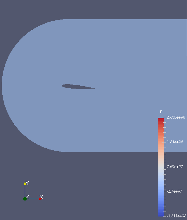
Visualization of the grid at a polynomial degree of p=2 just before terminating:
<Screenshot_2016-11-29_14-04-05.png>
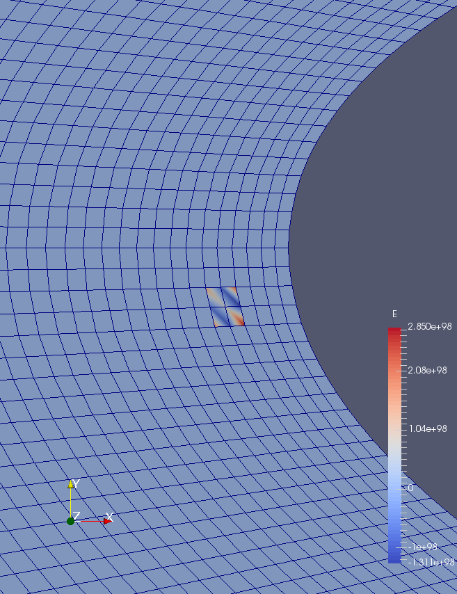
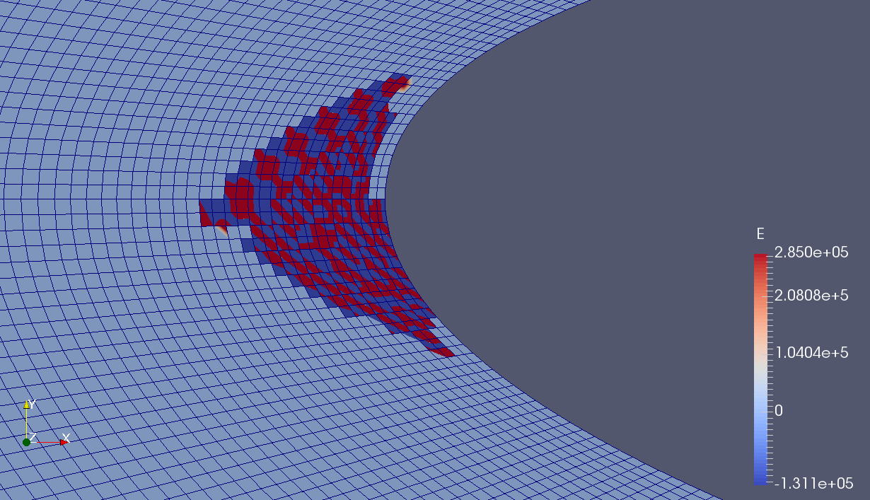
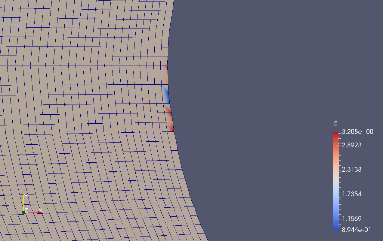
With auto-scale: <Screenshot from 2016-11-29 14-27-59.png>
Same solution with scaling by user: <Screenshot from 2016-11-29 15-33-10.png>
Please take into account the scaling above.
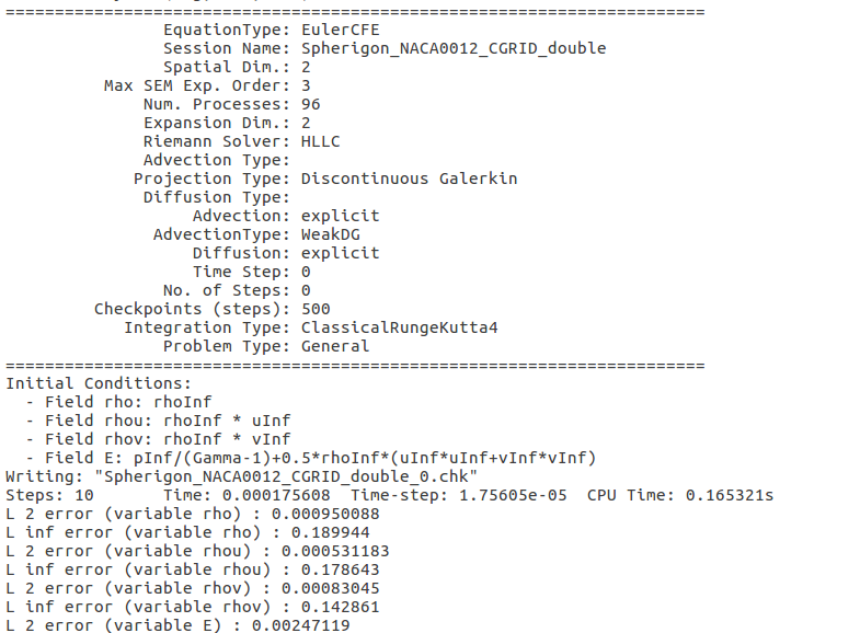
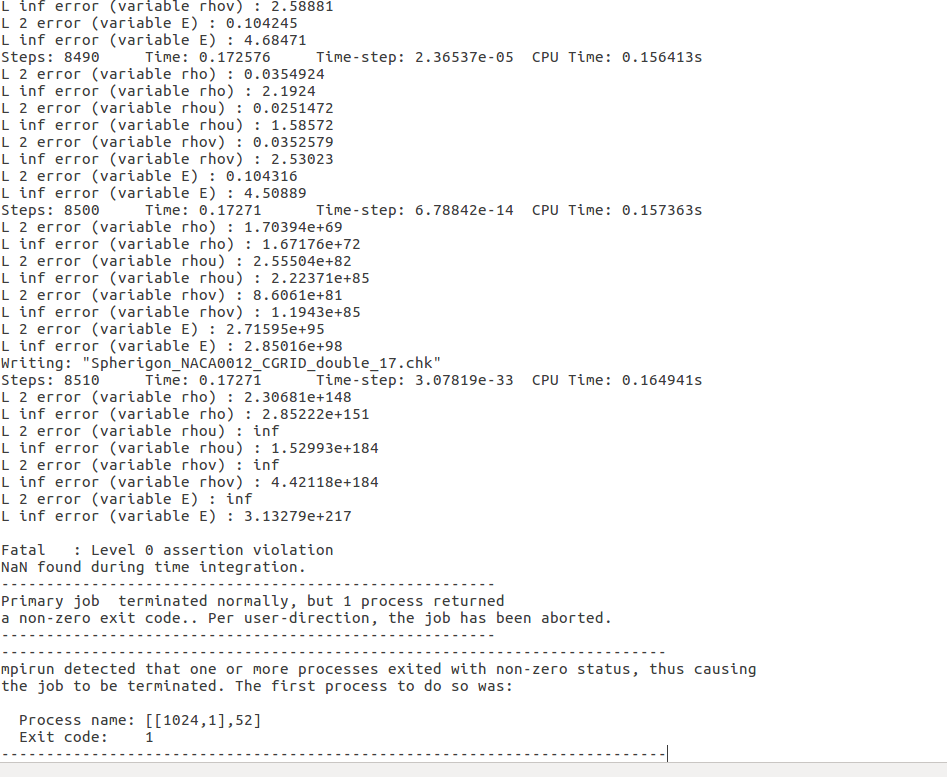
Error and conditions for example p=2:
<Screenshot from 2016-11-29 14-32-53.png> <Screenshot from 2016-11-29 14-33-22.png> <Screenshot from 2016-11-29 14-33-38.png>
Visualization of the grid at a polynomial degree of p=7 just before terminating:
<Screenshot from 2016-11-29 16-18-39.png>
(a few time steps after that the simulation terminates and the values go against inf...)
_______________________________________________ Nektar-users mailing list Nektar-users@imperial.ac.uk https://mailman.ic.ac.uk/mailman/listinfo/nektar-users
-- David Moxey (Research and Teaching Fellow) d.moxey@imperial.ac.uk | www.imperial.ac.uk/people/d.moxey Room 364, Department of Aeronautics, Imperial College London, London, SW7 2AZ, UK.
Hi Dave, Hi Gianmarco, thanks for your answer. Yes I have already tried some mesh refinement, but either the time step is getting horrible small or it still terminates. I tested the expansion type, but it does not help (still termination). Actually I am thinking about starting with lower initial conditions and increasing them step by step. Maybe this helps. In addition to it some input from Gianmarco or a working example at a high Reynoldsnumber with the CompressibleFlowSolver would be great. Thanks in advance. Best regards Fabian ________________________________________ Von: David Moxey [d.moxey@imperial.ac.uk] Gesendet: Montag, 5. Dezember 2016 11:20 An: Selbach, Fabian Cc: Serson, Douglas; nektar-users@imperial.ac.uk Betreff: Re: [Nektar-users] Nonphysical terminated simulation - CompressibleFlowSolver Hi Fabian, Thanks for getting in touch and apologies for the slow response. I have a few thoughts that might help. - I would say that from your pictures, the meshes look very coarse, so you could definitely try some additional refinement. - Another source of instability can arise through the default quadrature points being used for inner products etc. You might find that using a more consistent integration could help, particularly if the grid is not well resolved. Depending on your mesh and setup, you can use an expansion tag like: <E COMPOSITE=“C[0]” BASISTYPE=“Modified_A,Modified_A" NUMMODES="3,3" POINTSTYPE="GaussLobattoLegendre,GaussLobattoLegendre" NUMPOINTS="6,6" FIELDS="rho,rhou,rhov,E" /> Note that this would use a polynomial order of 2 (nummodes = 3) whilst using double the number of grid points for integration (numpoints = 6) -- the default is one extra (numpoints = 4) which is generally sufficient but in the case of marginal resolution may lead to significant aliasing error. It'll therefore be more expensive but may be more robust. - I am not sure our CFL estimate for the compressible solver is all that great, so I would probably stick to a constant timestep, at least in the short term to investigate the reason for this instability. This is something we need to work on. - You should be aware that for these explicit schemes, larger polynomial orders will have a greater impact on the size of the maximum timestep, so perhaps best to limit to p=3-5 -- p=7 might be a bit restrictive on the timestep. It is probably better to try a grid refinement rather than increase the polynomial order. If none of this helps we can also see if Gianmarco has some input since he has run these cases extensively during his PhD and encountered may similar problems! Cheers, Dave
On 2 Dec 2016, at 09:53, Selbach, Fabian <fabian.selbach@student.uni-siegen.de> wrote:
Hi Douglas, Dear users,
thanks for your explanation of the EulerADCFE.
Your hint to decrease the CFL does not help to stabilize the simulation. Also decreasing the time step on my own to a very small one (analogical CFL=0.4) and to use another time integration method makes no difference. The simulation terminates at the same time. But I observed, that using less CPUs for parallel simulation helps to remain stable for a longer time, but finally it terminates too. Could it be a problem due to parallelization?
I will try to generate a new and better grid, because this is the last clue I got.
Has somebody else an idea what could causes this oscillations?
Thanks in advance!
Best regards
Fabian Von: Serson, Douglas [d.serson14@imperial.ac.uk] Gesendet: Mittwoch, 30. November 2016 15:17 An: Selbach, Fabian; nektar-users Betreff: Re: [Nektar-users] Nonphysical terminated simulation - CompressibleFlowSolver
Hi Fabian,
I don't know what is causing these oscillations (maybe you need a lower CFL), but regarding your other question: EulerADCFE allows using artificial diffusion for shock capture, while EulerCFE is just the standard Euler solver. For EulerADCFE you need to set the "ShockCaptureType" property (possible values are "Smooth" and "NonSmooth") and the parameters described in section 9.4.1 of the user guide.
In the most recent version of the master branch (this was changed just a few days ago), it is also possible to use shock capture directly with EulerCFE. In this newer version, EulerCFE and EulerADCFE are the same thing, with the second name kept for backwards compatibility.
Cheers, Douglas From: nektar-users-bounces@imperial.ac.uk <nektar-users-bounces@imperial.ac.uk> on behalf of Selbach, Fabian <fabian.selbach@student.uni-siegen.de> Sent: 30 November 2016 13:21:42 To: nektar-users Subject: [Nektar-users] Nonphysical terminated simulation - CompressibleFlowSolver
Dear users,
I hope you can help one more time. I got nonphysical oscillations during my airfoil-simulation. At that time my simulations terminate with the message: "NaN found during time integration". For more information of the error and parameters see pictures below. I tried to solve this by a higher polynomial degree up to p=7 (this generates 1.5 Mio grid-points here for a 2D simulation), but the simulation terminates still. The time step itself is computed by a fixed CFL=0.9 condition. Maybe this is the wrong way, because this condition is not sufficient?
So please can somebody give me a hint about that? Do I have to use another kind of grid, because the resolution of the boundary at the peak of the airfoil is not high enough or the grid lines have no be orthogonal to the surface? I am already using the spherigons-tool and tried to get a smooth boundary of my airfoil.
I am using the CompressibleFlowSolver on a parallel run up to 96 CPUs by solving the Euler-Equations (EulerCFE) and the Navier-Stokes-Equations (NavierStokesCFE). The simulation terminates for both.
By the way what is the difference between EulerCFE and EulerADCFE (there are no information about it anywhere)? I tried to run the example NACA0012 of the paper "Nektar++: An open-source spectral/hp element framework". The conditions use the EulerADCFE, but by running this example the simulation does not terminate, but also does not change (values of every variable in the whole domain are constant over the time - no changes?).
Thanks for any help!
Best regards
Fabian
Visualization of the grid at a polynomial degree of p=2 just before terminating:
<Screenshot_2016-11-29_14-04-05.png>
With auto-scale: <Screenshot from 2016-11-29 14-27-59.png>
Same solution with scaling by user: <Screenshot from 2016-11-29 15-33-10.png>
Please take into account the scaling above.
Error and conditions for example p=2:
<Screenshot from 2016-11-29 14-32-53.png> <Screenshot from 2016-11-29 14-33-22.png> <Screenshot from 2016-11-29 14-33-38.png>
Visualization of the grid at a polynomial degree of p=7 just before terminating:
<Screenshot from 2016-11-29 16-18-39.png>
(a few time steps after that the simulation terminates and the values go against inf...)
_______________________________________________ Nektar-users mailing list Nektar-users@imperial.ac.uk https://mailman.ic.ac.uk/mailman/listinfo/nektar-users
-- David Moxey (Research and Teaching Fellow) d.moxey@imperial.ac.uk | www.imperial.ac.uk/people/d.moxey Room 364, Department of Aeronautics, Imperial College London, London, SW7 2AZ, UK.
Hi Fabian, can you try with a constant dt that satisfies the CFL condition (i.e. take the one plotted at the first few time-steps when using the CFL tool and decrease it by one order of magnitude). Also, I think that your proposed strategy of starting with a lower IC might help. Finally, are you running DG-collocated? If so, I suggest you increase the number of quadrature points. while keeping the same polynomial order. You can find more details on this topic here: http://www.sciencedirect.com/science/article/pii/S0021999115004301 Let me know if this helps! Best, Gianmarco Gianmarco Mengaldo Department of Aeronautics and Mathematics Room 730/731, Huxley Building Imperial College London South Kensington Campus London SW7 2AZ M: +447462029290 On Dec 5, 2016, at 9:35 AM, Selbach, Fabian <fabian.selbach@student.uni-siegen.de<mailto:fabian.selbach@student.uni-siegen.de>> wrote: Hi Dave, Hi Gianmarco, thanks for your answer. Yes I have already tried some mesh refinement, but either the time step is getting horrible small or it still terminates. I tested the expansion type, but it does not help (still termination). Actually I am thinking about starting with lower initial conditions and increasing them step by step. Maybe this helps. In addition to it some input from Gianmarco or a working example at a high Reynoldsnumber with the CompressibleFlowSolver would be great. Thanks in advance. Best regards Fabian ________________________________________ Von: David Moxey [d.moxey@imperial.ac.uk<mailto:d.moxey@imperial.ac.uk>] Gesendet: Montag, 5. Dezember 2016 11:20 An: Selbach, Fabian Cc: Serson, Douglas; nektar-users@imperial.ac.uk<mailto:nektar-users@imperial.ac.uk> Betreff: Re: [Nektar-users] Nonphysical terminated simulation - CompressibleFlowSolver Hi Fabian, Thanks for getting in touch and apologies for the slow response. I have a few thoughts that might help. - I would say that from your pictures, the meshes look very coarse, so you could definitely try some additional refinement. - Another source of instability can arise through the default quadrature points being used for inner products etc. You might find that using a more consistent integration could help, particularly if the grid is not well resolved. Depending on your mesh and setup, you can use an expansion tag like: <E COMPOSITE=“C[0]” BASISTYPE=“Modified_A,Modified_A" NUMMODES="3,3" POINTSTYPE="GaussLobattoLegendre,GaussLobattoLegendre" NUMPOINTS="6,6" FIELDS="rho,rhou,rhov,E" /> Note that this would use a polynomial order of 2 (nummodes = 3) whilst using double the number of grid points for integration (numpoints = 6) -- the default is one extra (numpoints = 4) which is generally sufficient but in the case of marginal resolution may lead to significant aliasing error. It'll therefore be more expensive but may be more robust. - I am not sure our CFL estimate for the compressible solver is all that great, so I would probably stick to a constant timestep, at least in the short term to investigate the reason for this instability. This is something we need to work on. - You should be aware that for these explicit schemes, larger polynomial orders will have a greater impact on the size of the maximum timestep, so perhaps best to limit to p=3-5 -- p=7 might be a bit restrictive on the timestep. It is probably better to try a grid refinement rather than increase the polynomial order. If none of this helps we can also see if Gianmarco has some input since he has run these cases extensively during his PhD and encountered may similar problems! Cheers, Dave On 2 Dec 2016, at 09:53, Selbach, Fabian <fabian.selbach@student.uni-siegen.de<mailto:fabian.selbach@student.uni-siegen.de>> wrote: Hi Douglas, Dear users, thanks for your explanation of the EulerADCFE. Your hint to decrease the CFL does not help to stabilize the simulation. Also decreasing the time step on my own to a very small one (analogical CFL=0.4) and to use another time integration method makes no difference. The simulation terminates at the same time. But I observed, that using less CPUs for parallel simulation helps to remain stable for a longer time, but finally it terminates too. Could it be a problem due to parallelization? I will try to generate a new and better grid, because this is the last clue I got. Has somebody else an idea what could causes this oscillations? Thanks in advance! Best regards Fabian Von: Serson, Douglas [d.serson14@imperial.ac.uk<mailto:d.serson14@imperial.ac.uk>] Gesendet: Mittwoch, 30. November 2016 15:17 An: Selbach, Fabian; nektar-users Betreff: Re: [Nektar-users] Nonphysical terminated simulation - CompressibleFlowSolver Hi Fabian, I don't know what is causing these oscillations (maybe you need a lower CFL), but regarding your other question: EulerADCFE allows using artificial diffusion for shock capture, while EulerCFE is just the standard Euler solver. For EulerADCFE you need to set the "ShockCaptureType" property (possible values are "Smooth" and "NonSmooth") and the parameters described in section 9.4.1 of the user guide. In the most recent version of the master branch (this was changed just a few days ago), it is also possible to use shock capture directly with EulerCFE. In this newer version, EulerCFE and EulerADCFE are the same thing, with the second name kept for backwards compatibility. Cheers, Douglas From: nektar-users-bounces@imperial.ac.uk<mailto:nektar-users-bounces@imperial.ac.uk> <nektar-users-bounces@imperial.ac.uk<mailto:nektar-users-bounces@imperial.ac.uk>> on behalf of Selbach, Fabian <fabian.selbach@student.uni-siegen.de<mailto:fabian.selbach@student.uni-siegen.de>> Sent: 30 November 2016 13:21:42 To: nektar-users Subject: [Nektar-users] Nonphysical terminated simulation - CompressibleFlowSolver Dear users, I hope you can help one more time. I got nonphysical oscillations during my airfoil-simulation. At that time my simulations terminate with the message: "NaN found during time integration". For more information of the error and parameters see pictures below. I tried to solve this by a higher polynomial degree up to p=7 (this generates 1.5 Mio grid-points here for a 2D simulation), but the simulation terminates still. The time step itself is computed by a fixed CFL=0.9 condition. Maybe this is the wrong way, because this condition is not sufficient? So please can somebody give me a hint about that? Do I have to use another kind of grid, because the resolution of the boundary at the peak of the airfoil is not high enough or the grid lines have no be orthogonal to the surface? I am already using the spherigons-tool and tried to get a smooth boundary of my airfoil. I am using the CompressibleFlowSolver on a parallel run up to 96 CPUs by solving the Euler-Equations (EulerCFE) and the Navier-Stokes-Equations (NavierStokesCFE). The simulation terminates for both. By the way what is the difference between EulerCFE and EulerADCFE (there are no information about it anywhere)? I tried to run the example NACA0012 of the paper "Nektar++: An open-source spectral/hp element framework". The conditions use the EulerADCFE, but by running this example the simulation does not terminate, but also does not change (values of every variable in the whole domain are constant over the time - no changes?). Thanks for any help! Best regards Fabian Visualization of the grid at a polynomial degree of p=2 just before terminating: <Screenshot_2016-11-29_14-04-05.png> With auto-scale: <Screenshot from 2016-11-29 14-27-59.png> Same solution with scaling by user: <Screenshot from 2016-11-29 15-33-10.png> Please take into account the scaling above. Error and conditions for example p=2: <Screenshot from 2016-11-29 14-32-53.png> <Screenshot from 2016-11-29 14-33-22.png> <Screenshot from 2016-11-29 14-33-38.png> Visualization of the grid at a polynomial degree of p=7 just before terminating: <Screenshot from 2016-11-29 16-18-39.png> (a few time steps after that the simulation terminates and the values go against inf...) _______________________________________________ Nektar-users mailing list Nektar-users@imperial.ac.uk<mailto:Nektar-users@imperial.ac.uk> https://mailman.ic.ac.uk/mailman/listinfo/nektar-users -- David Moxey (Research and Teaching Fellow) d.moxey@imperial.ac.uk<mailto:d.moxey@imperial.ac.uk> | www.imperial.ac.uk/people/d.moxey<http://www.imperial.ac.uk/people/d.moxey> Room 364, Department of Aeronautics, Imperial College London, London, SW7 2AZ, UK.
Hi Gianmarco, thanks for your answer. Decreasing the CFL condition does not help. Neither using a very low CFL, nor using a constant dt. Starting with a lower IC helps only in terms of using a lower Re. Higher Re terminates, so I think it must be a problem due to physics. By running DG-collocated you mean using an expansion tag like: <E COMPOSITE=“C[0]” BASISTYPE=“Modified_A,Modified_A" NUMMODES="3,3" POINTSTYPE="GaussLobattoLegendre,GaussLobattoLegendre" NUMPOINTS="6,6" FIELDS="rho,rhou,rhov,E" /> ? Yes I tried that what you mentioned in the paper, but it does not help. Finally using a polynomial degree of p=1 and a relative coarse mesh (I refined every time at the points of oscillation after termination) helps to run the simulation (actually until dimensionless t=14) , but with very bad accuracy. After increasing p = 2 with the same mesh it terminates again after t<1. Of course I adjust the time-step. So it seems that there must be an addiction between the resolution of the mesh and the possible polynomial degree? Is this the case? Is there actually a way to do a LES or is the only possibility to use an unresolved DNS? Best regards Fabian ________________________________ Von: Mengaldo, Gianmarco [g.mengaldo11@imperial.ac.uk] Gesendet: Montag, 12. Dezember 2016 18:50 An: Selbach, Fabian Cc: Moxey, David; Mengaldo, Gianmarco; Serson, Douglas; nektar-users Betreff: Re: [Nektar-users] Nonphysical terminated simulation - CompressibleFlowSolver Hi Fabian, can you try with a constant dt that satisfies the CFL condition (i.e. take the one plotted at the first few time-steps when using the CFL tool and decrease it by one order of magnitude). Also, I think that your proposed strategy of starting with a lower IC might help. Finally, are you running DG-collocated? If so, I suggest you increase the number of quadrature points. while keeping the same polynomial order. You can find more details on this topic here: http://www.sciencedirect.com/science/article/pii/S0021999115004301 Let me know if this helps! Best, Gianmarco Gianmarco Mengaldo Department of Aeronautics and Mathematics Room 730/731, Huxley Building Imperial College London South Kensington Campus London SW7 2AZ M: +447462029290 On Dec 5, 2016, at 9:35 AM, Selbach, Fabian <fabian.selbach@student.uni-siegen.de<mailto:fabian.selbach@student.uni-siegen.de>> wrote: Hi Dave, Hi Gianmarco, thanks for your answer. Yes I have already tried some mesh refinement, but either the time step is getting horrible small or it still terminates. I tested the expansion type, but it does not help (still termination). Actually I am thinking about starting with lower initial conditions and increasing them step by step. Maybe this helps. In addition to it some input from Gianmarco or a working example at a high Reynoldsnumber with the CompressibleFlowSolver would be great. Thanks in advance. Best regards Fabian ________________________________________ Von: David Moxey [d.moxey@imperial.ac.uk<mailto:d.moxey@imperial.ac.uk>] Gesendet: Montag, 5. Dezember 2016 11:20 An: Selbach, Fabian Cc: Serson, Douglas; nektar-users@imperial.ac.uk<mailto:nektar-users@imperial.ac.uk> Betreff: Re: [Nektar-users] Nonphysical terminated simulation - CompressibleFlowSolver Hi Fabian, Thanks for getting in touch and apologies for the slow response. I have a few thoughts that might help. - I would say that from your pictures, the meshes look very coarse, so you could definitely try some additional refinement. - Another source of instability can arise through the default quadrature points being used for inner products etc. You might find that using a more consistent integration could help, particularly if the grid is not well resolved. Depending on your mesh and setup, you can use an expansion tag like: <E COMPOSITE=“C[0]” BASISTYPE=“Modified_A,Modified_A" NUMMODES="3,3" POINTSTYPE="GaussLobattoLegendre,GaussLobattoLegendre" NUMPOINTS="6,6" FIELDS="rho,rhou,rhov,E" /> Note that this would use a polynomial order of 2 (nummodes = 3) whilst using double the number of grid points for integration (numpoints = 6) -- the default is one extra (numpoints = 4) which is generally sufficient but in the case of marginal resolution may lead to significant aliasing error. It'll therefore be more expensive but may be more robust. - I am not sure our CFL estimate for the compressible solver is all that great, so I would probably stick to a constant timestep, at least in the short term to investigate the reason for this instability. This is something we need to work on. - You should be aware that for these explicit schemes, larger polynomial orders will have a greater impact on the size of the maximum timestep, so perhaps best to limit to p=3-5 -- p=7 might be a bit restrictive on the timestep. It is probably better to try a grid refinement rather than increase the polynomial order. If none of this helps we can also see if Gianmarco has some input since he has run these cases extensively during his PhD and encountered may similar problems! Cheers, Dave On 2 Dec 2016, at 09:53, Selbach, Fabian <fabian.selbach@student.uni-siegen.de<mailto:fabian.selbach@student.uni-siegen.de>> wrote: Hi Douglas, Dear users, thanks for your explanation of the EulerADCFE. Your hint to decrease the CFL does not help to stabilize the simulation. Also decreasing the time step on my own to a very small one (analogical CFL=0.4) and to use another time integration method makes no difference. The simulation terminates at the same time. But I observed, that using less CPUs for parallel simulation helps to remain stable for a longer time, but finally it terminates too. Could it be a problem due to parallelization? I will try to generate a new and better grid, because this is the last clue I got. Has somebody else an idea what could causes this oscillations? Thanks in advance! Best regards Fabian Von: Serson, Douglas [d.serson14@imperial.ac.uk<mailto:d.serson14@imperial.ac.uk>] Gesendet: Mittwoch, 30. November 2016 15:17 An: Selbach, Fabian; nektar-users Betreff: Re: [Nektar-users] Nonphysical terminated simulation - CompressibleFlowSolver Hi Fabian, I don't know what is causing these oscillations (maybe you need a lower CFL), but regarding your other question: EulerADCFE allows using artificial diffusion for shock capture, while EulerCFE is just the standard Euler solver. For EulerADCFE you need to set the "ShockCaptureType" property (possible values are "Smooth" and "NonSmooth") and the parameters described in section 9.4.1 of the user guide. In the most recent version of the master branch (this was changed just a few days ago), it is also possible to use shock capture directly with EulerCFE. In this newer version, EulerCFE and EulerADCFE are the same thing, with the second name kept for backwards compatibility. Cheers, Douglas From: nektar-users-bounces@imperial.ac.uk<mailto:nektar-users-bounces@imperial.ac.uk> <nektar-users-bounces@imperial.ac.uk<mailto:nektar-users-bounces@imperial.ac.uk>> on behalf of Selbach, Fabian <fabian.selbach@student.uni-siegen.de<mailto:fabian.selbach@student.uni-siegen.de>> Sent: 30 November 2016 13:21:42 To: nektar-users Subject: [Nektar-users] Nonphysical terminated simulation - CompressibleFlowSolver Dear users, I hope you can help one more time. I got nonphysical oscillations during my airfoil-simulation. At that time my simulations terminate with the message: "NaN found during time integration". For more information of the error and parameters see pictures below. I tried to solve this by a higher polynomial degree up to p=7 (this generates 1.5 Mio grid-points here for a 2D simulation), but the simulation terminates still. The time step itself is computed by a fixed CFL=0.9 condition. Maybe this is the wrong way, because this condition is not sufficient? So please can somebody give me a hint about that? Do I have to use another kind of grid, because the resolution of the boundary at the peak of the airfoil is not high enough or the grid lines have no be orthogonal to the surface? I am already using the spherigons-tool and tried to get a smooth boundary of my airfoil. I am using the CompressibleFlowSolver on a parallel run up to 96 CPUs by solving the Euler-Equations (EulerCFE) and the Navier-Stokes-Equations (NavierStokesCFE). The simulation terminates for both. By the way what is the difference between EulerCFE and EulerADCFE (there are no information about it anywhere)? I tried to run the example NACA0012 of the paper "Nektar++: An open-source spectral/hp element framework". The conditions use the EulerADCFE, but by running this example the simulation does not terminate, but also does not change (values of every variable in the whole domain are constant over the time - no changes?). Thanks for any help! Best regards Fabian Visualization of the grid at a polynomial degree of p=2 just before terminating: <Screenshot_2016-11-29_14-04-05.png> With auto-scale: <Screenshot from 2016-11-29 14-27-59.png> Same solution with scaling by user: <Screenshot from 2016-11-29 15-33-10.png> Please take into account the scaling above. Error and conditions for example p=2: <Screenshot from 2016-11-29 14-32-53.png> <Screenshot from 2016-11-29 14-33-22.png> <Screenshot from 2016-11-29 14-33-38.png> Visualization of the grid at a polynomial degree of p=7 just before terminating: <Screenshot from 2016-11-29 16-18-39.png> (a few time steps after that the simulation terminates and the values go against inf...) _______________________________________________ Nektar-users mailing list Nektar-users@imperial.ac.uk<mailto:Nektar-users@imperial.ac.uk> https://mailman.ic.ac.uk/mailman/listinfo/nektar-users -- David Moxey (Research and Teaching Fellow) d.moxey@imperial.ac.uk<mailto:d.moxey@imperial.ac.uk> | www.imperial.ac.uk/people/d.moxey<http://www.imperial.ac.uk/people/d.moxey> Room 364, Department of Aeronautics, Imperial College London, London, SW7 2AZ, UK.
Does it blow up at the leading edge every time? Sent from my iPhone On Dec 15, 2016, at 5:09 AM, Selbach, Fabian <fabian.selbach@student.uni-siegen.de<mailto:fabian.selbach@student.uni-siegen.de>> wrote: Hi Gianmarco, thanks for your answer. Decreasing the CFL condition does not help. Neither using a very low CFL, nor using a constant dt. Starting with a lower IC helps only in terms of using a lower Re. Higher Re terminates, so I think it must be a problem due to physics. By running DG-collocated you mean using an expansion tag like: <E COMPOSITE=“C[0]” BASISTYPE=“Modified_A,Modified_A" NUMMODES="3,3" POINTSTYPE="GaussLobattoLegendre,GaussLobattoLegendre" NUMPOINTS="6,6" FIELDS="rho,rhou,rhov,E" /> ? Yes I tried that what you mentioned in the paper, but it does not help. Finally using a polynomial degree of p=1 and a relative coarse mesh (I refined every time at the points of oscillation after termination) helps to run the simulation (actually until dimensionless t=14) , but with very bad accuracy. After increasing p = 2 with the same mesh it terminates again after t<1. Of course I adjust the time-step. So it seems that there must be an addiction between the resolution of the mesh and the possible polynomial degree? Is this the case? Is there actually a way to do a LES or is the only possibility to use an unresolved DNS? Best regards Fabian ________________________________ Von: Mengaldo, Gianmarco [g.mengaldo11@imperial.ac.uk<mailto:g.mengaldo11@imperial.ac.uk>] Gesendet: Montag, 12. Dezember 2016 18:50 An: Selbach, Fabian Cc: Moxey, David; Mengaldo, Gianmarco; Serson, Douglas; nektar-users Betreff: Re: [Nektar-users] Nonphysical terminated simulation - CompressibleFlowSolver Hi Fabian, can you try with a constant dt that satisfies the CFL condition (i.e. take the one plotted at the first few time-steps when using the CFL tool and decrease it by one order of magnitude). Also, I think that your proposed strategy of starting with a lower IC might help. Finally, are you running DG-collocated? If so, I suggest you increase the number of quadrature points. while keeping the same polynomial order. You can find more details on this topic here: http://www.sciencedirect.com/science/article/pii/S0021999115004301 Let me know if this helps! Best, Gianmarco Gianmarco Mengaldo Department of Aeronautics and Mathematics Room 730/731, Huxley Building Imperial College London South Kensington Campus London SW7 2AZ M: +447462029290 On Dec 5, 2016, at 9:35 AM, Selbach, Fabian <fabian.selbach@student.uni-siegen.de<mailto:fabian.selbach@student.uni-siegen.de>> wrote: Hi Dave, Hi Gianmarco, thanks for your answer. Yes I have already tried some mesh refinement, but either the time step is getting horrible small or it still terminates. I tested the expansion type, but it does not help (still termination). Actually I am thinking about starting with lower initial conditions and increasing them step by step. Maybe this helps. In addition to it some input from Gianmarco or a working example at a high Reynoldsnumber with the CompressibleFlowSolver would be great. Thanks in advance. Best regards Fabian ________________________________________ Von: David Moxey [d.moxey@imperial.ac.uk<mailto:d.moxey@imperial.ac.uk>] Gesendet: Montag, 5. Dezember 2016 11:20 An: Selbach, Fabian Cc: Serson, Douglas; nektar-users@imperial.ac.uk<mailto:nektar-users@imperial.ac.uk> Betreff: Re: [Nektar-users] Nonphysical terminated simulation - CompressibleFlowSolver Hi Fabian, Thanks for getting in touch and apologies for the slow response. I have a few thoughts that might help. - I would say that from your pictures, the meshes look very coarse, so you could definitely try some additional refinement. - Another source of instability can arise through the default quadrature points being used for inner products etc. You might find that using a more consistent integration could help, particularly if the grid is not well resolved. Depending on your mesh and setup, you can use an expansion tag like: <E COMPOSITE=“C[0]” BASISTYPE=“Modified_A,Modified_A" NUMMODES="3,3" POINTSTYPE="GaussLobattoLegendre,GaussLobattoLegendre" NUMPOINTS="6,6" FIELDS="rho,rhou,rhov,E" /> Note that this would use a polynomial order of 2 (nummodes = 3) whilst using double the number of grid points for integration (numpoints = 6) -- the default is one extra (numpoints = 4) which is generally sufficient but in the case of marginal resolution may lead to significant aliasing error. It'll therefore be more expensive but may be more robust. - I am not sure our CFL estimate for the compressible solver is all that great, so I would probably stick to a constant timestep, at least in the short term to investigate the reason for this instability. This is something we need to work on. - You should be aware that for these explicit schemes, larger polynomial orders will have a greater impact on the size of the maximum timestep, so perhaps best to limit to p=3-5 -- p=7 might be a bit restrictive on the timestep. It is probably better to try a grid refinement rather than increase the polynomial order. If none of this helps we can also see if Gianmarco has some input since he has run these cases extensively during his PhD and encountered may similar problems! Cheers, Dave On 2 Dec 2016, at 09:53, Selbach, Fabian <fabian.selbach@student.uni-siegen.de<mailto:fabian.selbach@student.uni-siegen.de>> wrote: Hi Douglas, Dear users, thanks for your explanation of the EulerADCFE. Your hint to decrease the CFL does not help to stabilize the simulation. Also decreasing the time step on my own to a very small one (analogical CFL=0.4) and to use another time integration method makes no difference. The simulation terminates at the same time. But I observed, that using less CPUs for parallel simulation helps to remain stable for a longer time, but finally it terminates too. Could it be a problem due to parallelization? I will try to generate a new and better grid, because this is the last clue I got. Has somebody else an idea what could causes this oscillations? Thanks in advance! Best regards Fabian Von: Serson, Douglas [d.serson14@imperial.ac.uk<mailto:d.serson14@imperial.ac.uk>] Gesendet: Mittwoch, 30. November 2016 15:17 An: Selbach, Fabian; nektar-users Betreff: Re: [Nektar-users] Nonphysical terminated simulation - CompressibleFlowSolver Hi Fabian, I don't know what is causing these oscillations (maybe you need a lower CFL), but regarding your other question: EulerADCFE allows using artificial diffusion for shock capture, while EulerCFE is just the standard Euler solver. For EulerADCFE you need to set the "ShockCaptureType" property (possible values are "Smooth" and "NonSmooth") and the parameters described in section 9.4.1 of the user guide. In the most recent version of the master branch (this was changed just a few days ago), it is also possible to use shock capture directly with EulerCFE. In this newer version, EulerCFE and EulerADCFE are the same thing, with the second name kept for backwards compatibility. Cheers, Douglas From: nektar-users-bounces@imperial.ac.uk<mailto:nektar-users-bounces@imperial.ac.uk> <nektar-users-bounces@imperial.ac.uk<mailto:nektar-users-bounces@imperial.ac.uk>> on behalf of Selbach, Fabian <fabian.selbach@student.uni-siegen.de<mailto:fabian.selbach@student.uni-siegen.de>> Sent: 30 November 2016 13:21:42 To: nektar-users Subject: [Nektar-users] Nonphysical terminated simulation - CompressibleFlowSolver Dear users, I hope you can help one more time. I got nonphysical oscillations during my airfoil-simulation. At that time my simulations terminate with the message: "NaN found during time integration". For more information of the error and parameters see pictures below. I tried to solve this by a higher polynomial degree up to p=7 (this generates 1.5 Mio grid-points here for a 2D simulation), but the simulation terminates still. The time step itself is computed by a fixed CFL=0.9 condition. Maybe this is the wrong way, because this condition is not sufficient? So please can somebody give me a hint about that? Do I have to use another kind of grid, because the resolution of the boundary at the peak of the airfoil is not high enough or the grid lines have no be orthogonal to the surface? I am already using the spherigons-tool and tried to get a smooth boundary of my airfoil. I am using the CompressibleFlowSolver on a parallel run up to 96 CPUs by solving the Euler-Equations (EulerCFE) and the Navier-Stokes-Equations (NavierStokesCFE). The simulation terminates for both. By the way what is the difference between EulerCFE and EulerADCFE (there are no information about it anywhere)? I tried to run the example NACA0012 of the paper "Nektar++: An open-source spectral/hp element framework". The conditions use the EulerADCFE, but by running this example the simulation does not terminate, but also does not change (values of every variable in the whole domain are constant over the time - no changes?). Thanks for any help! Best regards Fabian Visualization of the grid at a polynomial degree of p=2 just before terminating: <Screenshot_2016-11-29_14-04-05.png> With auto-scale: <Screenshot from 2016-11-29 14-27-59.png> Same solution with scaling by user: <Screenshot from 2016-11-29 15-33-10.png> Please take into account the scaling above. Error and conditions for example p=2: <Screenshot from 2016-11-29 14-32-53.png> <Screenshot from 2016-11-29 14-33-22.png> <Screenshot from 2016-11-29 14-33-38.png> Visualization of the grid at a polynomial degree of p=7 just before terminating: <Screenshot from 2016-11-29 16-18-39.png> (a few time steps after that the simulation terminates and the values go against inf...) _______________________________________________ Nektar-users mailing list Nektar-users@imperial.ac.uk<mailto:Nektar-users@imperial.ac.uk> https://mailman.ic.ac.uk/mailman/listinfo/nektar-users -- David Moxey (Research and Teaching Fellow) d.moxey@imperial.ac.uk<mailto:d.moxey@imperial.ac.uk> | www.imperial.ac.uk/people/d.moxey<http://www.imperial.ac.uk/people/d.moxey> Room 364, Department of Aeronautics, Imperial College London, London, SW7 2AZ, UK.
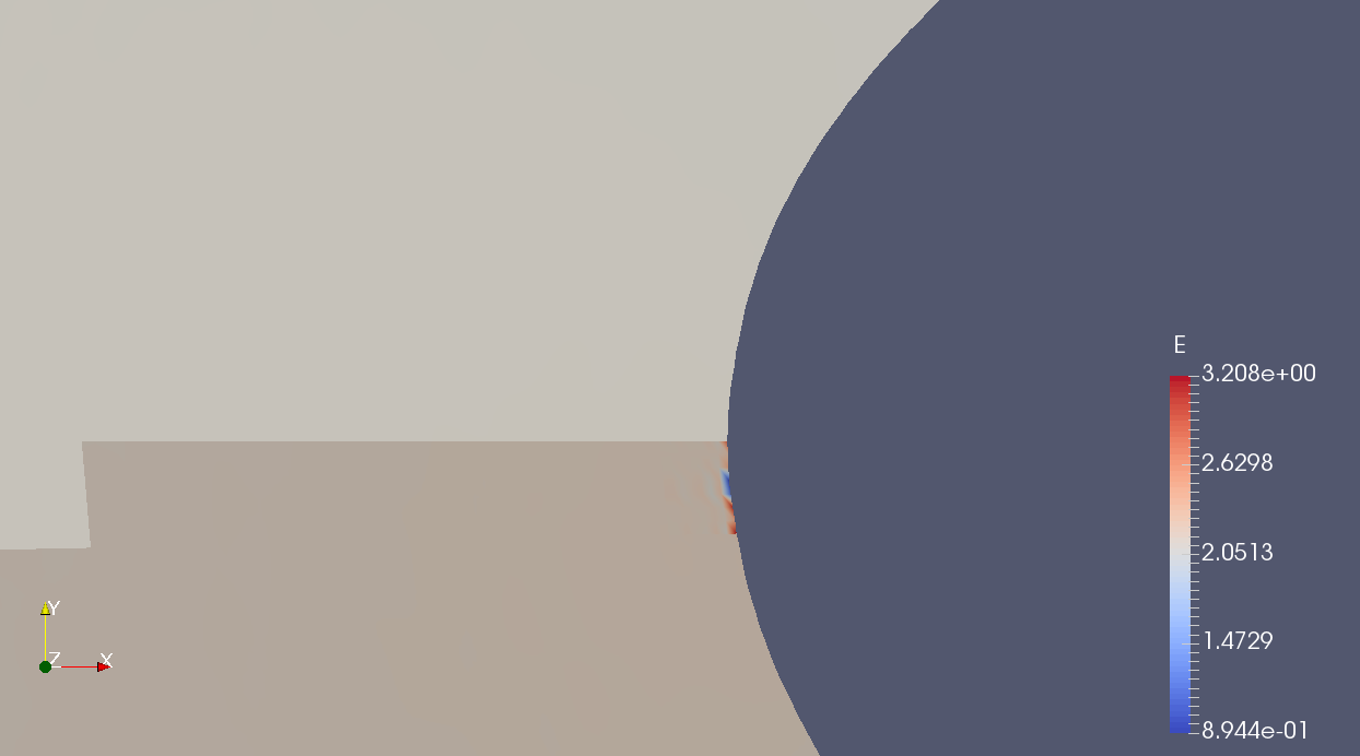
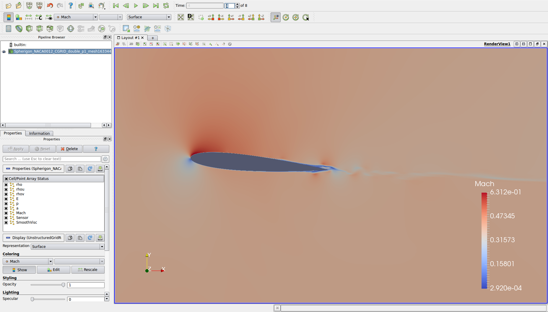
Hi Gianmarco, it depends on. The simulation with p=1 and finally t=14 terminates at the trailing edge. I refined the mesh there and right no it still works, but with very bad accuracy. See picture below. The simulation with p=2 produces oscillations at different points - also at the leading edge, but besides at the top and bottom of the airfoil, but always next to the boundary. I am still refining the mesh there, but getting many grid-points and an awful small time step... So it seems a higher polynomial degree causes more oscillations and needs to have a finer grid. Is this true? Is it because of the higher resolution of a higher polynomial degree? So I can resolve smaller waves, but they can cause more oscillations? Best regards Fabian Simulation of NACA0012, Ma=0.4, Re=408000, p=1: [cid:c096bca1-daa3-4b6c-8459-aad62e765caa] ________________________________ Von: Mengaldo, Gianmarco [g.mengaldo11@imperial.ac.uk] Gesendet: Donnerstag, 15. Dezember 2016 18:29 An: Selbach, Fabian Cc: Moxey, David; Serson, Douglas; nektar-users Betreff: Re: AW: [Nektar-users] Nonphysical terminated simulation - CompressibleFlowSolver Does it blow up at the leading edge every time? Sent from my iPhone On Dec 15, 2016, at 5:09 AM, Selbach, Fabian <fabian.selbach@student.uni-siegen.de<mailto:fabian.selbach@student.uni-siegen.de>> wrote: Hi Gianmarco, thanks for your answer. Decreasing the CFL condition does not help. Neither using a very low CFL, nor using a constant dt. Starting with a lower IC helps only in terms of using a lower Re. Higher Re terminates, so I think it must be a problem due to physics. By running DG-collocated you mean using an expansion tag like: <E COMPOSITE=“C[0]” BASISTYPE=“Modified_A,Modified_A" NUMMODES="3,3" POINTSTYPE="GaussLobattoLegendre,GaussLobattoLegendre" NUMPOINTS="6,6" FIELDS="rho,rhou,rhov,E" /> ? Yes I tried that what you mentioned in the paper, but it does not help. Finally using a polynomial degree of p=1 and a relative coarse mesh (I refined every time at the points of oscillation after termination) helps to run the simulation (actually until dimensionless t=14) , but with very bad accuracy. After increasing p = 2 with the same mesh it terminates again after t<1. Of course I adjust the time-step. So it seems that there must be an addiction between the resolution of the mesh and the possible polynomial degree? Is this the case? Is there actually a way to do a LES or is the only possibility to use an unresolved DNS? Best regards Fabian ________________________________ Von: Mengaldo, Gianmarco [g.mengaldo11@imperial.ac.uk<mailto:g.mengaldo11@imperial.ac.uk>] Gesendet: Montag, 12. Dezember 2016 18:50 An: Selbach, Fabian Cc: Moxey, David; Mengaldo, Gianmarco; Serson, Douglas; nektar-users Betreff: Re: [Nektar-users] Nonphysical terminated simulation - CompressibleFlowSolver Hi Fabian, can you try with a constant dt that satisfies the CFL condition (i.e. take the one plotted at the first few time-steps when using the CFL tool and decrease it by one order of magnitude). Also, I think that your proposed strategy of starting with a lower IC might help. Finally, are you running DG-collocated? If so, I suggest you increase the number of quadrature points. while keeping the same polynomial order. You can find more details on this topic here: http://www.sciencedirect.com/science/article/pii/S0021999115004301 Let me know if this helps! Best, Gianmarco Gianmarco Mengaldo Department of Aeronautics and Mathematics Room 730/731, Huxley Building Imperial College London South Kensington Campus London SW7 2AZ M: +447462029290 On Dec 5, 2016, at 9:35 AM, Selbach, Fabian <fabian.selbach@student.uni-siegen.de<mailto:fabian.selbach@student.uni-siegen.de>> wrote: Hi Dave, Hi Gianmarco, thanks for your answer. Yes I have already tried some mesh refinement, but either the time step is getting horrible small or it still terminates. I tested the expansion type, but it does not help (still termination). Actually I am thinking about starting with lower initial conditions and increasing them step by step. Maybe this helps. In addition to it some input from Gianmarco or a working example at a high Reynoldsnumber with the CompressibleFlowSolver would be great. Thanks in advance. Best regards Fabian ________________________________________ Von: David Moxey [d.moxey@imperial.ac.uk<mailto:d.moxey@imperial.ac.uk>] Gesendet: Montag, 5. Dezember 2016 11:20 An: Selbach, Fabian Cc: Serson, Douglas; nektar-users@imperial.ac.uk<mailto:nektar-users@imperial.ac.uk> Betreff: Re: [Nektar-users] Nonphysical terminated simulation - CompressibleFlowSolver Hi Fabian, Thanks for getting in touch and apologies for the slow response. I have a few thoughts that might help. - I would say that from your pictures, the meshes look very coarse, so you could definitely try some additional refinement. - Another source of instability can arise through the default quadrature points being used for inner products etc. You might find that using a more consistent integration could help, particularly if the grid is not well resolved. Depending on your mesh and setup, you can use an expansion tag like: <E COMPOSITE=“C[0]” BASISTYPE=“Modified_A,Modified_A" NUMMODES="3,3" POINTSTYPE="GaussLobattoLegendre,GaussLobattoLegendre" NUMPOINTS="6,6" FIELDS="rho,rhou,rhov,E" /> Note that this would use a polynomial order of 2 (nummodes = 3) whilst using double the number of grid points for integration (numpoints = 6) -- the default is one extra (numpoints = 4) which is generally sufficient but in the case of marginal resolution may lead to significant aliasing error. It'll therefore be more expensive but may be more robust. - I am not sure our CFL estimate for the compressible solver is all that great, so I would probably stick to a constant timestep, at least in the short term to investigate the reason for this instability. This is something we need to work on. - You should be aware that for these explicit schemes, larger polynomial orders will have a greater impact on the size of the maximum timestep, so perhaps best to limit to p=3-5 -- p=7 might be a bit restrictive on the timestep. It is probably better to try a grid refinement rather than increase the polynomial order. If none of this helps we can also see if Gianmarco has some input since he has run these cases extensively during his PhD and encountered may similar problems! Cheers, Dave On 2 Dec 2016, at 09:53, Selbach, Fabian <fabian.selbach@student.uni-siegen.de<mailto:fabian.selbach@student.uni-siegen.de>> wrote: Hi Douglas, Dear users, thanks for your explanation of the EulerADCFE. Your hint to decrease the CFL does not help to stabilize the simulation. Also decreasing the time step on my own to a very small one (analogical CFL=0.4) and to use another time integration method makes no difference. The simulation terminates at the same time. But I observed, that using less CPUs for parallel simulation helps to remain stable for a longer time, but finally it terminates too. Could it be a problem due to parallelization? I will try to generate a new and better grid, because this is the last clue I got. Has somebody else an idea what could causes this oscillations? Thanks in advance! Best regards Fabian Von: Serson, Douglas [d.serson14@imperial.ac.uk<mailto:d.serson14@imperial.ac.uk>] Gesendet: Mittwoch, 30. November 2016 15:17 An: Selbach, Fabian; nektar-users Betreff: Re: [Nektar-users] Nonphysical terminated simulation - CompressibleFlowSolver Hi Fabian, I don't know what is causing these oscillations (maybe you need a lower CFL), but regarding your other question: EulerADCFE allows using artificial diffusion for shock capture, while EulerCFE is just the standard Euler solver. For EulerADCFE you need to set the "ShockCaptureType" property (possible values are "Smooth" and "NonSmooth") and the parameters described in section 9.4.1 of the user guide. In the most recent version of the master branch (this was changed just a few days ago), it is also possible to use shock capture directly with EulerCFE. In this newer version, EulerCFE and EulerADCFE are the same thing, with the second name kept for backwards compatibility. Cheers, Douglas From: nektar-users-bounces@imperial.ac.uk<mailto:nektar-users-bounces@imperial.ac.uk> <nektar-users-bounces@imperial.ac.uk<mailto:nektar-users-bounces@imperial.ac.uk>> on behalf of Selbach, Fabian <fabian.selbach@student.uni-siegen.de<mailto:fabian.selbach@student.uni-siegen.de>> Sent: 30 November 2016 13:21:42 To: nektar-users Subject: [Nektar-users] Nonphysical terminated simulation - CompressibleFlowSolver Dear users, I hope you can help one more time. I got nonphysical oscillations during my airfoil-simulation. At that time my simulations terminate with the message: "NaN found during time integration". For more information of the error and parameters see pictures below. I tried to solve this by a higher polynomial degree up to p=7 (this generates 1.5 Mio grid-points here for a 2D simulation), but the simulation terminates still. The time step itself is computed by a fixed CFL=0.9 condition. Maybe this is the wrong way, because this condition is not sufficient? So please can somebody give me a hint about that? Do I have to use another kind of grid, because the resolution of the boundary at the peak of the airfoil is not high enough or the grid lines have no be orthogonal to the surface? I am already using the spherigons-tool and tried to get a smooth boundary of my airfoil. I am using the CompressibleFlowSolver on a parallel run up to 96 CPUs by solving the Euler-Equations (EulerCFE) and the Navier-Stokes-Equations (NavierStokesCFE). The simulation terminates for both. By the way what is the difference between EulerCFE and EulerADCFE (there are no information about it anywhere)? I tried to run the example NACA0012 of the paper "Nektar++: An open-source spectral/hp element framework". The conditions use the EulerADCFE, but by running this example the simulation does not terminate, but also does not change (values of every variable in the whole domain are constant over the time - no changes?). Thanks for any help! Best regards Fabian Visualization of the grid at a polynomial degree of p=2 just before terminating: <Screenshot_2016-11-29_14-04-05.png> With auto-scale: <Screenshot from 2016-11-29 14-27-59.png> Same solution with scaling by user: <Screenshot from 2016-11-29 15-33-10.png> Please take into account the scaling above. Error and conditions for example p=2: <Screenshot from 2016-11-29 14-32-53.png> <Screenshot from 2016-11-29 14-33-22.png> <Screenshot from 2016-11-29 14-33-38.png> Visualization of the grid at a polynomial degree of p=7 just before terminating: <Screenshot from 2016-11-29 16-18-39.png> (a few time steps after that the simulation terminates and the values go against inf...) _______________________________________________ Nektar-users mailing list Nektar-users@imperial.ac.uk<mailto:Nektar-users@imperial.ac.uk> https://mailman.ic.ac.uk/mailman/listinfo/nektar-users -- David Moxey (Research and Teaching Fellow) d.moxey@imperial.ac.uk<mailto:d.moxey@imperial.ac.uk> | www.imperial.ac.uk/people/d.moxey<http://www.imperial.ac.uk/people/d.moxey> Room 364, Department of Aeronautics, Imperial College London, London, SW7 2AZ, UK.
Hi Fabian, Is this a 2D simulation? The Reynolds number your are trying to simulate is very high, so you likely need to add some drain (i.e. SVV) in the simulation. The fact that P = 1 somehow works is likely related to the diffusivity of the scheme. I guess that you might need to look into an SVV-type drain that is already implemented into the library. Cheers, Gian On Dec 16, 2016, at 3:12 AM, Selbach, Fabian <fabian.selbach@student.uni-siegen.de<mailto:fabian.selbach@student.uni-siegen.de>> wrote: Hi Gianmarco, it depends on. The simulation with p=1 and finally t=14 terminates at the trailing edge. I refined the mesh there and right no it still works, but with very bad accuracy. See picture below. The simulation with p=2 produces oscillations at different points - also at the leading edge, but besides at the top and bottom of the airfoil, but always next to the boundary. I am still refining the mesh there, but getting many grid-points and an awful small time step... So it seems a higher polynomial degree causes more oscillations and needs to have a finer grid. Is this true? Is it because of the higher resolution of a higher polynomial degree? So I can resolve smaller waves, but they can cause more oscillations? Best regards Fabian Simulation of NACA0012, Ma=0.4, Re=408000, p=1: <Screenshot from 2016-12-16 11-43-36.png> ________________________________ Von: Mengaldo, Gianmarco [g.mengaldo11@imperial.ac.uk<mailto:g.mengaldo11@imperial.ac.uk>] Gesendet: Donnerstag, 15. Dezember 2016 18:29 An: Selbach, Fabian Cc: Moxey, David; Serson, Douglas; nektar-users Betreff: Re: AW: [Nektar-users] Nonphysical terminated simulation - CompressibleFlowSolver Does it blow up at the leading edge every time? Sent from my iPhone On Dec 15, 2016, at 5:09 AM, Selbach, Fabian <fabian.selbach@student.uni-siegen.de<mailto:fabian.selbach@student.uni-siegen.de>> wrote: Hi Gianmarco, thanks for your answer. Decreasing the CFL condition does not help. Neither using a very low CFL, nor using a constant dt. Starting with a lower IC helps only in terms of using a lower Re. Higher Re terminates, so I think it must be a problem due to physics. By running DG-collocated you mean using an expansion tag like: <E COMPOSITE=“C[0]” BASISTYPE=“Modified_A,Modified_A" NUMMODES="3,3" POINTSTYPE="GaussLobattoLegendre,GaussLobattoLegendre" NUMPOINTS="6,6" FIELDS="rho,rhou,rhov,E" /> ? Yes I tried that what you mentioned in the paper, but it does not help. Finally using a polynomial degree of p=1 and a relative coarse mesh (I refined every time at the points of oscillation after termination) helps to run the simulation (actually until dimensionless t=14) , but with very bad accuracy. After increasing p = 2 with the same mesh it terminates again after t<1. Of course I adjust the time-step. So it seems that there must be an addiction between the resolution of the mesh and the possible polynomial degree? Is this the case? Is there actually a way to do a LES or is the only possibility to use an unresolved DNS? Best regards Fabian ________________________________ Von: Mengaldo, Gianmarco [g.mengaldo11@imperial.ac.uk<mailto:g.mengaldo11@imperial.ac.uk>] Gesendet: Montag, 12. Dezember 2016 18:50 An: Selbach, Fabian Cc: Moxey, David; Mengaldo, Gianmarco; Serson, Douglas; nektar-users Betreff: Re: [Nektar-users] Nonphysical terminated simulation - CompressibleFlowSolver Hi Fabian, can you try with a constant dt that satisfies the CFL condition (i.e. take the one plotted at the first few time-steps when using the CFL tool and decrease it by one order of magnitude). Also, I think that your proposed strategy of starting with a lower IC might help. Finally, are you running DG-collocated? If so, I suggest you increase the number of quadrature points. while keeping the same polynomial order. You can find more details on this topic here: http://www.sciencedirect.com/science/article/pii/S0021999115004301 Let me know if this helps! Best, Gianmarco Gianmarco Mengaldo Department of Aeronautics and Mathematics Room 730/731, Huxley Building Imperial College London South Kensington Campus London SW7 2AZ M: +447462029290 On Dec 5, 2016, at 9:35 AM, Selbach, Fabian <fabian.selbach@student.uni-siegen.de<mailto:fabian.selbach@student.uni-siegen.de>> wrote: Hi Dave, Hi Gianmarco, thanks for your answer. Yes I have already tried some mesh refinement, but either the time step is getting horrible small or it still terminates. I tested the expansion type, but it does not help (still termination). Actually I am thinking about starting with lower initial conditions and increasing them step by step. Maybe this helps. In addition to it some input from Gianmarco or a working example at a high Reynoldsnumber with the CompressibleFlowSolver would be great. Thanks in advance. Best regards Fabian ________________________________________ Von: David Moxey [d.moxey@imperial.ac.uk<mailto:d.moxey@imperial.ac.uk>] Gesendet: Montag, 5. Dezember 2016 11:20 An: Selbach, Fabian Cc: Serson, Douglas; nektar-users@imperial.ac.uk<mailto:nektar-users@imperial.ac.uk> Betreff: Re: [Nektar-users] Nonphysical terminated simulation - CompressibleFlowSolver Hi Fabian, Thanks for getting in touch and apologies for the slow response. I have a few thoughts that might help. - I would say that from your pictures, the meshes look very coarse, so you could definitely try some additional refinement. - Another source of instability can arise through the default quadrature points being used for inner products etc. You might find that using a more consistent integration could help, particularly if the grid is not well resolved. Depending on your mesh and setup, you can use an expansion tag like: <E COMPOSITE=“C[0]” BASISTYPE=“Modified_A,Modified_A" NUMMODES="3,3" POINTSTYPE="GaussLobattoLegendre,GaussLobattoLegendre" NUMPOINTS="6,6" FIELDS="rho,rhou,rhov,E" /> Note that this would use a polynomial order of 2 (nummodes = 3) whilst using double the number of grid points for integration (numpoints = 6) -- the default is one extra (numpoints = 4) which is generally sufficient but in the case of marginal resolution may lead to significant aliasing error. It'll therefore be more expensive but may be more robust. - I am not sure our CFL estimate for the compressible solver is all that great, so I would probably stick to a constant timestep, at least in the short term to investigate the reason for this instability. This is something we need to work on. - You should be aware that for these explicit schemes, larger polynomial orders will have a greater impact on the size of the maximum timestep, so perhaps best to limit to p=3-5 -- p=7 might be a bit restrictive on the timestep. It is probably better to try a grid refinement rather than increase the polynomial order. If none of this helps we can also see if Gianmarco has some input since he has run these cases extensively during his PhD and encountered may similar problems! Cheers, Dave On 2 Dec 2016, at 09:53, Selbach, Fabian <fabian.selbach@student.uni-siegen.de<mailto:fabian.selbach@student.uni-siegen.de>> wrote: Hi Douglas, Dear users, thanks for your explanation of the EulerADCFE. Your hint to decrease the CFL does not help to stabilize the simulation. Also decreasing the time step on my own to a very small one (analogical CFL=0.4) and to use another time integration method makes no difference. The simulation terminates at the same time. But I observed, that using less CPUs for parallel simulation helps to remain stable for a longer time, but finally it terminates too. Could it be a problem due to parallelization? I will try to generate a new and better grid, because this is the last clue I got. Has somebody else an idea what could causes this oscillations? Thanks in advance! Best regards Fabian Von: Serson, Douglas [d.serson14@imperial.ac.uk<mailto:d.serson14@imperial.ac.uk>] Gesendet: Mittwoch, 30. November 2016 15:17 An: Selbach, Fabian; nektar-users Betreff: Re: [Nektar-users] Nonphysical terminated simulation - CompressibleFlowSolver Hi Fabian, I don't know what is causing these oscillations (maybe you need a lower CFL), but regarding your other question: EulerADCFE allows using artificial diffusion for shock capture, while EulerCFE is just the standard Euler solver. For EulerADCFE you need to set the "ShockCaptureType" property (possible values are "Smooth" and "NonSmooth") and the parameters described in section 9.4.1 of the user guide. In the most recent version of the master branch (this was changed just a few days ago), it is also possible to use shock capture directly with EulerCFE. In this newer version, EulerCFE and EulerADCFE are the same thing, with the second name kept for backwards compatibility. Cheers, Douglas From: nektar-users-bounces@imperial.ac.uk<mailto:nektar-users-bounces@imperial.ac.uk> <nektar-users-bounces@imperial.ac.uk<mailto:nektar-users-bounces@imperial.ac.uk>> on behalf of Selbach, Fabian <fabian.selbach@student.uni-siegen.de<mailto:fabian.selbach@student.uni-siegen.de>> Sent: 30 November 2016 13:21:42 To: nektar-users Subject: [Nektar-users] Nonphysical terminated simulation - CompressibleFlowSolver Dear users, I hope you can help one more time. I got nonphysical oscillations during my airfoil-simulation. At that time my simulations terminate with the message: "NaN found during time integration". For more information of the error and parameters see pictures below. I tried to solve this by a higher polynomial degree up to p=7 (this generates 1.5 Mio grid-points here for a 2D simulation), but the simulation terminates still. The time step itself is computed by a fixed CFL=0.9 condition. Maybe this is the wrong way, because this condition is not sufficient? So please can somebody give me a hint about that? Do I have to use another kind of grid, because the resolution of the boundary at the peak of the airfoil is not high enough or the grid lines have no be orthogonal to the surface? I am already using the spherigons-tool and tried to get a smooth boundary of my airfoil. I am using the CompressibleFlowSolver on a parallel run up to 96 CPUs by solving the Euler-Equations (EulerCFE) and the Navier-Stokes-Equations (NavierStokesCFE). The simulation terminates for both. By the way what is the difference between EulerCFE and EulerADCFE (there are no information about it anywhere)? I tried to run the example NACA0012 of the paper "Nektar++: An open-source spectral/hp element framework". The conditions use the EulerADCFE, but by running this example the simulation does not terminate, but also does not change (values of every variable in the whole domain are constant over the time - no changes?). Thanks for any help! Best regards Fabian Visualization of the grid at a polynomial degree of p=2 just before terminating: <Screenshot_2016-11-29_14-04-05.png> With auto-scale: <Screenshot from 2016-11-29 14-27-59.png> Same solution with scaling by user: <Screenshot from 2016-11-29 15-33-10.png> Please take into account the scaling above. Error and conditions for example p=2: <Screenshot from 2016-11-29 14-32-53.png> <Screenshot from 2016-11-29 14-33-22.png> <Screenshot from 2016-11-29 14-33-38.png> Visualization of the grid at a polynomial degree of p=7 just before terminating: <Screenshot from 2016-11-29 16-18-39.png> (a few time steps after that the simulation terminates and the values go against inf...) _______________________________________________ Nektar-users mailing list Nektar-users@imperial.ac.uk<mailto:Nektar-users@imperial.ac.uk> https://mailman.ic.ac.uk/mailman/listinfo/nektar-users -- David Moxey (Research and Teaching Fellow) d.moxey@imperial.ac.uk<mailto:d.moxey@imperial.ac.uk> | www.imperial.ac.uk/people/d.moxey<http://www.imperial.ac.uk/people/d.moxey> Room 364, Department of Aeronautics, Imperial College London, London, SW7 2AZ, UK.
Hi Gian, yes this is a 2D Simulation. Finally I want to simulate in 3D. I will try to do add some SVV. Thank you. By the way is there a guide or an example how to implement the SVV in a NavierStokesCFE-Simulation? Best regards Fabian
Am 16.12.2016 um 12:12 schrieb Selbach, Fabian <fabian.selbach@student.uni-siegen.de>:
Hi Gianmarco,
it depends on. The simulation with p=1 and finally t=14 terminates at the trailing edge. I refined the mesh there and right no it still works, but with very bad accuracy. See picture below.
The simulation with p=2 produces oscillations at different points - also at the leading edge, but besides at the top and bottom of the airfoil, but always next to the boundary. I am still refining the mesh there, but getting many grid-points and an awful small time step...
So it seems a higher polynomial degree causes more oscillations and needs to have a finer grid. Is this true? Is it because of the higher resolution of a higher polynomial degree? So I can resolve smaller waves, but they can cause more oscillations?
Best regards
Fabian
Simulation of NACA0012, Ma=0.4, Re=408000, p=1:
<Screenshot from 2016-12-16 11-43-36.png>
Von: Mengaldo, Gianmarco [g.mengaldo11@imperial.ac.uk] Gesendet: Donnerstag, 15. Dezember 2016 18:29 An: Selbach, Fabian Cc: Moxey, David; Serson, Douglas; nektar-users Betreff: Re: AW: [Nektar-users] Nonphysical terminated simulation - CompressibleFlowSolver
Does it blow up at the leading edge every time?
Sent from my iPhone
On Dec 15, 2016, at 5:09 AM, Selbach, Fabian <fabian.selbach@student.uni-siegen.de> wrote:
Hi Gianmarco,
thanks for your answer.
Decreasing the CFL condition does not help. Neither using a very low CFL, nor using a constant dt.
Starting with a lower IC helps only in terms of using a lower Re. Higher Re terminates, so I think it must be a problem due to physics.
By running DG-collocated you mean using an expansion tag like:
<E COMPOSITE=“C[0]” BASISTYPE=“Modified_A,Modified_A" NUMMODES="3,3" POINTSTYPE="GaussLobattoLegendre,GaussLobattoLegendre" NUMPOINTS="6,6" FIELDS="rho,rhou,rhov,E" /> ? Yes I tried that what you mentioned in the paper, but it does not help.
Finally using a polynomial degree of p=1 and a relative coarse mesh (I refined every time at the points of oscillation after termination) helps to run the simulation (actually until dimensionless t=14) , but with very bad accuracy. After increasing p = 2 with the same mesh it terminates again after t<1. Of course I adjust the time-step. So it seems that there must be an addiction between the resolution of the mesh and the possible polynomial degree? Is this the case?
Is there actually a way to do a LES or is the only possibility to use an unresolved DNS?
Best regards Fabian
Von: Mengaldo, Gianmarco [g.mengaldo11@imperial.ac.uk] Gesendet: Montag, 12. Dezember 2016 18:50 An: Selbach, Fabian Cc: Moxey, David; Mengaldo, Gianmarco; Serson, Douglas; nektar-users Betreff: Re: [Nektar-users] Nonphysical terminated simulation - CompressibleFlowSolver
Hi Fabian,
can you try with a constant dt that satisfies the CFL condition (i.e. take the one plotted at the first few time-steps when using the CFL tool and decrease it by one order of magnitude).
Also, I think that your proposed strategy of starting with a lower IC might help.
Finally, are you running DG-collocated? If so, I suggest you increase the number of quadrature points. while keeping the same polynomial order. You can find more details on this topic here: http://www.sciencedirect.com/science/article/pii/S0021999115004301
Let me know if this helps!
Best, Gianmarco
Gianmarco Mengaldo Department of Aeronautics and Mathematics Room 730/731, Huxley Building Imperial College London South Kensington Campus London SW7 2AZ M: +447462029290
On Dec 5, 2016, at 9:35 AM, Selbach, Fabian <fabian.selbach@student.uni-siegen.de> wrote:
Hi Dave, Hi Gianmarco,
thanks for your answer. Yes I have already tried some mesh refinement, but either the time step is getting horrible small or it still terminates. I tested the expansion type, but it does not help (still termination).
Actually I am thinking about starting with lower initial conditions and increasing them step by step. Maybe this helps.
In addition to it some input from Gianmarco or a working example at a high Reynoldsnumber with the CompressibleFlowSolver would be great.
Thanks in advance.
Best regards
Fabian ________________________________________ Von: David Moxey [d.moxey@imperial.ac.uk] Gesendet: Montag, 5. Dezember 2016 11:20 An: Selbach, Fabian Cc: Serson, Douglas; nektar-users@imperial.ac.uk Betreff: Re: [Nektar-users] Nonphysical terminated simulation - CompressibleFlowSolver
Hi Fabian,
Thanks for getting in touch and apologies for the slow response. I have a few thoughts that might help.
- I would say that from your pictures, the meshes look very coarse, so you could definitely try some additional refinement.
- Another source of instability can arise through the default quadrature points being used for inner products etc. You might find that using a more consistent integration could help, particularly if the grid is not well resolved. Depending on your mesh and setup, you can use an expansion tag like:
<E COMPOSITE=“C[0]” BASISTYPE=“Modified_A,Modified_A" NUMMODES="3,3" POINTSTYPE="GaussLobattoLegendre,GaussLobattoLegendre" NUMPOINTS="6,6" FIELDS="rho,rhou,rhov,E" />
Note that this would use a polynomial order of 2 (nummodes = 3) whilst using double the number of grid points for integration (numpoints = 6) -- the default is one extra (numpoints = 4) which is generally sufficient but in the case of marginal resolution may lead to significant aliasing error. It'll therefore be more expensive but may be more robust.
- I am not sure our CFL estimate for the compressible solver is all that great, so I would probably stick to a constant timestep, at least in the short term to investigate the reason for this instability. This is something we need to work on.
- You should be aware that for these explicit schemes, larger polynomial orders will have a greater impact on the size of the maximum timestep, so perhaps best to limit to p=3-5 -- p=7 might be a bit restrictive on the timestep. It is probably better to try a grid refinement rather than increase the polynomial order.
If none of this helps we can also see if Gianmarco has some input since he has run these cases extensively during his PhD and encountered may similar problems!
Cheers,
Dave
On 2 Dec 2016, at 09:53, Selbach, Fabian <fabian.selbach@student.uni-siegen.de> wrote:
Hi Douglas, Dear users,
thanks for your explanation of the EulerADCFE.
Your hint to decrease the CFL does not help to stabilize the simulation. Also decreasing the time step on my own to a very small one (analogical CFL=0.4) and to use another time integration method makes no difference. The simulation terminates at the same time. But I observed, that using less CPUs for parallel simulation helps to remain stable for a longer time, but finally it terminates too. Could it be a problem due to parallelization?
I will try to generate a new and better grid, because this is the last clue I got.
Has somebody else an idea what could causes this oscillations?
Thanks in advance!
Best regards
Fabian Von: Serson, Douglas [d.serson14@imperial.ac.uk] Gesendet: Mittwoch, 30. November 2016 15:17 An: Selbach, Fabian; nektar-users Betreff: Re: [Nektar-users] Nonphysical terminated simulation - CompressibleFlowSolver
Hi Fabian,
I don't know what is causing these oscillations (maybe you need a lower CFL), but regarding your other question: EulerADCFE allows using artificial diffusion for shock capture, while EulerCFE is just the standard Euler solver. For EulerADCFE you need to set the "ShockCaptureType" property (possible values are "Smooth" and "NonSmooth") and the parameters described in section 9.4.1 of the user guide.
In the most recent version of the master branch (this was changed just a few days ago), it is also possible to use shock capture directly with EulerCFE. In this newer version, EulerCFE and EulerADCFE are the same thing, with the second name kept for backwards compatibility.
Cheers, Douglas From: nektar-users-bounces@imperial.ac.uk <nektar-users-bounces@imperial.ac.uk> on behalf of Selbach, Fabian <fabian.selbach@student.uni-siegen.de> Sent: 30 November 2016 13:21:42 To: nektar-users Subject: [Nektar-users] Nonphysical terminated simulation - CompressibleFlowSolver
Dear users,
I hope you can help one more time. I got nonphysical oscillations during my airfoil-simulation. At that time my simulations terminate with the message: "NaN found during time integration". For more information of the error and parameters see pictures below. I tried to solve this by a higher polynomial degree up to p=7 (this generates 1.5 Mio grid-points here for a 2D simulation), but the simulation terminates still. The time step itself is computed by a fixed CFL=0.9 condition. Maybe this is the wrong way, because this condition is not sufficient?
So please can somebody give me a hint about that? Do I have to use another kind of grid, because the resolution of the boundary at the peak of the airfoil is not high enough or the grid lines have no be orthogonal to the surface? I am already using the spherigons-tool and tried to get a smooth boundary of my airfoil.
I am using the CompressibleFlowSolver on a parallel run up to 96 CPUs by solving the Euler-Equations (EulerCFE) and the Navier-Stokes-Equations (NavierStokesCFE). The simulation terminates for both.
By the way what is the difference between EulerCFE and EulerADCFE (there are no information about it anywhere)? I tried to run the example NACA0012 of the paper "Nektar++: An open-source spectral/hp element framework". The conditions use the EulerADCFE, but by running this example the simulation does not terminate, but also does not change (values of every variable in the whole domain are constant over the time - no changes?).
Thanks for any help!
Best regards
Fabian
Visualization of the grid at a polynomial degree of p=2 just before terminating:
<Screenshot_2016-11-29_14-04-05.png>
With auto-scale: <Screenshot from 2016-11-29 14-27-59.png>
Same solution with scaling by user: <Screenshot from 2016-11-29 15-33-10.png>
Please take into account the scaling above.
Error and conditions for example p=2:
<Screenshot from 2016-11-29 14-32-53.png> <Screenshot from 2016-11-29 14-33-22.png> <Screenshot from 2016-11-29 14-33-38.png>
Visualization of the grid at a polynomial degree of p=7 just before terminating:
<Screenshot from 2016-11-29 16-18-39.png>
(a few time steps after that the simulation terminates and the values go against inf...)
_______________________________________________ Nektar-users mailing list Nektar-users@imperial.ac.uk https://mailman.ic.ac.uk/mailman/listinfo/nektar-users
-- David Moxey (Research and Teaching Fellow) d.moxey@imperial.ac.uk | www.imperial.ac.uk/people/d.moxey
Room 364, Department of Aeronautics, Imperial College London, London, SW7 2AZ, UK.
_______________________________________________ Nektar-users mailing list Nektar-users@imperial.ac.uk https://mailman.ic.ac.uk/mailman/listinfo/nektar-users
participants (5)
-
David Moxey
-
Fabian Selbach
-
Mengaldo, Gianmarco
-
Selbach, Fabian
-
Serson, Douglas